previous  home  next  PDF

4. Hamilton's Least Action Principle and Noether's Theorem

Michael Fowler, UVa

Beginnings of Dynamics

Galileo and Newton

Our text, Landau, begins (page 2!) by stating that the laws of dynamics come from the principle of least action, Hamilton’s principle. But where did Hamilton's principle come from?   He was certainly very familiar with the laws of dynamics as developed by Galileo and Newton, and in fact his principle follows directly from them—but it gives a new and valuable perspective. To see how this comes about, we'll briefly follow the historical path.

To begin, then, with Galileo. His two major contributions to dynamics were:

1. The realization, and experimental verification, that falling bodies have constant acceleration (provided air resistance can be ignored) and all falling bodies accelerate at the same rate. (This was the first step to Newton's law of universal gravitation.)

2. Galilean relativity: As he put it himself, if you are in a closed room below decks in a ship moving with steady velocity, no experiment on dropping or throwing something will look any different because of the ship’s motion: you can’t detect the motion.  As we would put it now, the laws of physics are the same in all inertial frames.

Newton’s major contributions were his laws of motion, and his law of universal gravitational attraction (which we'll discuss later).

His laws of motion are:

1. The law of inertia: A body moving at constant velocity will continue at that velocity unless acted on by a force.  (Actually, Galileo essentially stated this law, but just for a ball rolling on a horizontal plane, with zero frictional drag.)

2. $\overrightarrow{F}=m\overrightarrow{a}.$

3. Action = reaction.

In terms of Newton’s laws, Galilean relativity is clear: if the ship is moving at steady velocity $\overrightarrow{v}$ relative to the shore, than an object moving at $\overrightarrow{u}$ relative to the ship is moving at $\overrightarrow{u}+\overrightarrow{v}$ relative to the shore. If there is no force acting on the object, it is moving at steady velocity in both frames: both are inertial frames, defined as frames in which Newton’s first law holds.  And, since $\overrightarrow{v}$ is constant, the acceleration is the same in both frames, so if a force is introduced the second law is the same in the two frames.

(Needless to say, all this is classical, meaning nonrelativistic and of course nonquantum, mechanics.)

Newton's Laws Explain Everything (in Principle...)

...in a classical mechanical system. Any such system can be analyzed as a (possibly infinite) collection of parts, or particles, having defined mutual interactions, so in principle Newton’s laws—just in Cartesian coordinates—can provide a description of the motion evolving from any initial configuration of positions and velocities.

The problem is, though, that the equations are usually intractable—we can’t do the math.  In fact, the Cartesian coordinate positions and velocities might not be the best choice of parameters to specify the system’s configuration.  For example, a simple pendulum is obviously more naturally described by the angle the string makes with the vertical, as opposed to the Cartesian coordinates of the bob.  After Newton, a series of French mathematicians reformulated his laws in terms of more useful coordinates—culminating in Lagrange’s equations.

The Irish mathematician Hamilton then established that these improved dynamical equations could be derived using the calculus of variations to minimize an integral of a function, the Lagrangian, along a path in the system’s configuration space. 

This integral is called the action, so the rule is that the system follows the path of least action from the initial to the final configuration.

Nitpicking footnote: strictly, we need the path to be a stationary point in the space of possible paths, usually it's the least-action path.

From Newton’s Laws in Cartesian Co-ordinates to the Principle of Least Action

Calculus of Variations Done Backwards!

We’ve shown how (in lecture 2) given an integrand, we can find differential equations for the path in space time between two fixed points that minimizes the corresponding path integral between those points.

Now we’ll do the reverse: we already know the differential equations in Cartesian coordinates describing the path taken by a Newtonian particle in some potential. We’ll show how to use that knowledge to construct the integrand such that the action integral is a minimum along that path. (This follows Jeffreys and Jeffreys, Mathematical Physics.)

We begin with the simplest nontrivial system, a particle of mass $m$ moving in one dimension from one point to another in a specified time, we’ll assume it’s in a time-independent potential $U\left(x\right)$, so

$m\ddot{x}=-dU\left(x\right)/dx.$

Its path can be represented as a graph $x\left(t\right)$ against time$—$for example, for a ball thrown directly upwards in a constant gravitational field this would be a parabola.  

Initial and final positions are given: $x\left(t_1\right)=x_1$, $x\left(t_2\right)=x_2$, and the elapsed time is $t_2-t_1$.

 Notice we have not specified the initial velocity$—$we don’t have that option. The differential equation is only second order, so its solution is completely determined by the two (beginning and end) boundary conditions.

We’re now ready to embark on the calculus of variations in reverse.

Trivially, multiplying both sides of the equation of motion by an arbitrary infinitesimal function the equality still holds:

$m\ddot{x}\delta x\left(t\right)=-\left(dU\left(x\right)/dx\right)\delta x\left(t\right)$

and in fact if this equation is true for arbitrary $\delta x\left(t\right)$, the original equation of motion holds throughout, because we can always choose a $\delta x\left(t\right)$ nonzero only in the neighborhood of a particular time $t$, from which the original equation must be true at that $t$.

By analogy with Fermat’s principle in the preceding section, we can picture this $\delta x\left(t\right)$ as a slight variation in the path from the Newtonian trajectory, $x\left(t\right)\to x\left(t\right)+\delta x\left(t\right)$, and take the variation zero at the fixed ends, $\delta x\left(t_1\right)=\delta x\left(t_2\right)=0$. 

In Fermat’s (light wave) case, the integrated time elapsed along the path was minimized—there was zero change to first order on going from the (physical) path to a neighboring path. Developing the analogy, we’re looking for some dynamical quantity that has zero change to first order on going to a neighboring path having the same endpoints in space and time.   We’ve fixed the time, what’s left to integrate along the path?

For such a simple system, we don’t have many options!  As we’ve discussed above, the equation of motion is equivalent to (putting in an overall minus sign that will prove convenient)

${\displaystyle \underset{t_1}{\overset{t_2}{\int }}\left(-m\ddot{x}\left(t\right)-dU\left(x\left(t\right)\right)/dx\right)\delta x\left(t\right)}dt=0\text{to leading order, for all variations }\delta x\left(t\right).$

Integrating the first term by parts (recalling $\delta \left(x\right)=0$ at the endpoints):

$-{\displaystyle \underset{t_1}{\overset{t_2}{\int }}m\ddot{x}\left(t\right)\delta x\left(t\right)}dt={\displaystyle \underset{t_1}{\overset{t_2}{\int }}m\dot{x}\left(t\right)\delta \dot{x}\left(t\right)}dt={\displaystyle \underset{t_1}{\overset{t_2}{\int }}\delta \left(\frac{1}{2}m{\dot{x}}^2\left(t\right)\right)}dt={\displaystyle \underset{t_1}{\overset{t_2}{\int }}\delta T\left(x\left(t\right)\right)}dt$

using the standard notation $T$ for kinetic energy.

The second term integrates trivially:

$-{\displaystyle \underset{t_1}{\overset{t_2}{\int }}\left(dU\left(x\right)/dx\right)\delta x\left(t\right)dt}=-{\displaystyle \underset{t_1}{\overset{t_2}{\int }}\delta U\left(x\right)dt}$

establishing that on making an infinitesimal variation from the physical path (the one that satisfies Newton's laws) there is zero first order change in the integral of kinetic energy minus potential energy.

The standard notation is

$$\delta S=\delta {\displaystyle \underset{t_1}{\overset{t_2}{\int }}\left(T-U\right)dt=\delta }{\displaystyle \underset{t_1}{\overset{t_2}{\int }}Ldt=0.}$$

The integral $S$  is called the action integral, (also known as Hamilton’s Principal Function) and the integrand $T-U=L$ is called the Lagrangian.

This equation is Hamilton’s Principle of Least Action.

The derivation can be extended straightforwardly to a particle in three dimensions, in fact to $n$ interacting particles in three dimensions.  We shall assume that the forces on particles can be derived from potentials, including possibly time-dependent potentials, but we exclude frictional energy dissipation in this course. (It can be handled—see for example Vujanovic and Jones, Variational Methods in  Nonconservative Phenomena, Academic press, 1989.)

But Why Does It Follow This Path?

Fermat’s principle, that a light ray follows the path of least time, was easy to believe once it became clear that light was a wave.  The wave really propagates along all paths, and the phase change along a particular path is simply the time taken to travel that path measured in units of the light wave oscillation time. That means that if neighboring paths have the same length to first order the light waves along them will add coherently, otherwise they will interfere and essentially cancel.  So the path of least time is heavily favored, and when we look on a scale much greater than the wavelength of the light, we don’t even see the diffraction effects caused by imperfect cancellation, the light rays might as well be streams of particles, mysteriously choosing the path of least time.

So what has this to do with Hamilton’s principle?  Everything! A standard method in quantum mechanic is the so-called sum over paths, for example to find the probability amplitude for an electron to go from one point to another in a given time under a given potential, you can sum over all possible paths it might take, multiplying each path by a phase factor: and that phase factor (as established experimentally) is none other than Hamilton’s action integral divided by Planck’s constant, $S/\hslash .$  So, since all systems are really quantum systems, the classical limit $S\gg \hslash$  is a short-wavelength limit, in which the path of a dynamical system will be that of least action, exactly analogous to Fermat's principle for light waves. This is covered in my notes on Quantum Mechanics. The crucial insight was Dirac's, the method was developed by Feynman.

Bottom Line: All of classical mechanics follows from the Principle of Least Action. But that Principle itself follows from quantum mechanics!

Historical footnote:  Lagrange presented these methods in a classic book that Hamilton called a “scientific poem”.  Lagrange thought mechanics properly belonged to pure mathematics, it was a kind of geometry in four dimensions (space and time).  Hamilton was the first to use the principle of least action to derive Lagrange’s equations in the present form.  He built up the least action formalism directly from Fermat’s principle, considered in a medium where the velocity of light varies with position and with direction of the ray.  He saw mechanics as represented by geometrical optics in an appropriate space of higher dimensions.  But it didn’t apparently occur to him that this might be because it was really a wave theory!  (See Arnold, Mathematical Methods of Classical Mechanics, for details.)

Deriving Lagrange’s Equations from the Least Action Principle

Chooosing the Best Coordinates

We started with Newton’s equations of motion, expressed in Cartesian coordinates of particle positions. For many systems, these equations are mathematically intractable. Running the calculus of variations argument in reverse, we established Hamilton’s principle: the system moves along the path through configuration space for which the action integral, with integrand the Lagrangian $L=T-U,$ is a minimum.

We’re now free to begin from Hamilton’s principle, expressing the Lagrangian in variables that more naturally describe the system, taking advantage of any symmetries (such as using angle variables for rotationally invariant systems). Also, some forces do not need to be included in the description of the system: a simple pendulum is fully specified by its position and velocity, we do not need to know the tension in the string, although that would appear in a Newtonian analysis. The greater efficiency (and elegance) of the Lagrangian method, for most problems, will become evident on working through actual examples.

We’ll define a set of generalized coordinates $q=\left(q_1,\dots q_n\right)$ by requiring that they give a complete description of the configuration of the system (where everything is in space). The state of the system is specified by this set plus the corresponding velocities $\dot{q}=\left({\dot{q}}_1,\dots {\dot{q}}_n\right)$.

  For example, the $x$-coordinate of a particular particle $a$ is given by some function of the $q_i$ ’s, $x_a=f_{x_a}\left(q_1,\dots q_n\right),$ and the corresponding velocity component ${\dot{x}}_a={\displaystyle \sum _k\frac{\partial f_{x_a}}{\partial q_k}{\dot{q}}_k}$.

The Lagrangian will depend on all these variables in general, and also possibly on time explicitly, for example if there is a time-dependent external potential.  (But usually that isn’t the case.)

Hamilton’s principle gives

$\delta S=\delta {\displaystyle \underset{t_1}{\overset{t_2}{\int }}L\left(q_i,{\dot{q}}_i,t\right)}dt=0$

that is,

${\displaystyle \underset{t_1}{\overset{t_2}{\int }}{\displaystyle \sum _i\left(\frac{\partial L}{\partial q_i}\delta q_i+\frac{\partial L}{\partial {\dot{q}}_i}\delta {\dot{q}}_i\right)}}dt=0.$

Integrating by parts,

$\delta S={\left[{\displaystyle \sum _i\frac{\partial L}{\partial {\dot{q}}_i}\delta q_i}\right]}_{t_1}^{t_2}+{\displaystyle \underset{t_1}{\overset{t_2}{\int }}{\displaystyle \sum _i\left(\frac{\partial L}{\partial q_i}-\frac{d}{dt}\left(\frac{\partial L}{\partial {\dot{q}}_i}\right)\right)}}\delta q_{i}dt=0.$

Requiring the path deviation to be zero at the endpoints gives Lagrange’s equations:

$$\frac{d}{dt}\left(\frac{\partial L}{\partial {\dot{q}}_i}\right)-\frac{\partial L}{\partial q_i}=0.$$

Non-uniqueness of the Lagrangian

The Lagrangian is not uniquely defined: two Lagrangians differing by the total derivative with respect to time of some function will give the same identical equations on minimizing the action, 

$S^{\prime }={\displaystyle \underset{t_1}{\overset{t_2}{\int }}{L}^{\prime }\left(q,\dot{q},t\right)}dt={\displaystyle \underset{t_1}{\overset{t_2}{\int }}L\left(q,\dot{q},t\right)}dt+{\displaystyle \underset{t_1}{\overset{t_2}{\int }}\frac{df\left(q,t\right)}{dt}}dt=S+f\left(q\left(t_2\right),t_2\right)-f\left(q\left(t_1\right),t_1\right),$

and since $q\left(t_1\right),t_1,q\left(t_2\right),t_2$ are all fixed, the integral over $df/dt$ is trivially independent of path variations, and varying the path to minimize $S^{\prime }$ gives the same result as minimizing $S$. This turns out to be important later$—$it gives us a  useful new tool to change the variables in the Lagrangian.

First Integral:  Energy Conservation and the Hamiltonian

Since Lagrange’s equations are precisely a calculus of variations result, it follows from our earlier discussion that if the Lagrangian has no explicit time dependence then:

${\displaystyle \sum _i{\dot{q}}_i\frac{\partial L}{\partial {\dot{q}}_i}}-L=\text{constant}\text{.}$

(This is just the first integral $y^{\prime }\partial f/\partial y^{\prime }-f=\text{constant }$ discussed earlier, now with $n$ variables.)

This constant of motion is called the energy of the system, and denoted by $E$.  We say the energy is conserved, even in the presence of external potentials$—$provided those potentials are time-independent.

(We’ll just mention that the function on the left-hand side, ${\displaystyle \sum _i{\dot{q}}_i\partial L/\partial {\dot{q}}_i}-L,$ is the Hamiltonian. We don’t discuss it further at this point because, as we’ll find out, it is more naturally treated in other variables.)

We’ll now look at a couple of simple examples of the Lagrangian approach.

Example 1:  One Degree of Freedom: Atwood’s Machine

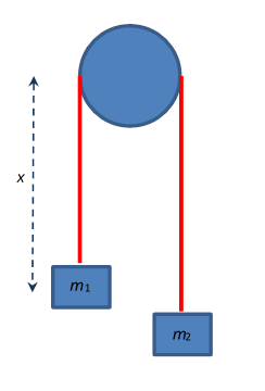
In 1784, the Rev. George Atwood, tutor at Trinity College, Cambridge, came up with a great demo for finding $g$.  It’s still with us.

The traditional Newtonian solution of this problem is to write $F=ma$ for the two masses, then eliminate the tension $T$. (To keep things simple, we’ll neglect the rotational inertia of the top pulley.)

The Lagrangian approach is, of course, to write down the Lagrangian, and derive the equation of motion.

Measuring gravitational potential energy from the top wheel axle, the potential energy is

$U\left(x\right)=-m_{1}gx-m_{2}g\left(\ell -x\right)$

and the Lagrangian

$L=T-U=\frac{1}{2}\left(m_1+m_2\right){\dot{x}}^2+m_{1}gx+m_{2}g\left(\ell -x\right).$

Lagrange’s equation:

$$\frac{d}{dt}\left(\frac{\partial L}{\partial \dot{x}}\right)-\frac{\partial L}{\partial x}=\left(m_1+m_2\right)\ddot{x}-\left(m_1-m_2\right)g=0$$

gives the equation of motion in just one step.

It’s usually pretty easy to figure out the kinetic energy and potential energy of a system, and thereby write down the Lagrangian. This is definitely less work than the Newtonian approach, which involves constraint forces, such as the tension in the string.  This force doesn’t even appear in the Lagrangian approach!  Other constraint forces, such as the normal force for a bead on a wire, or the normal force for a particle moving on a surface, or the tension in the string of a pendulum$—$none of these forces appear in the Lagrangian. Notice, though, that these forces never do any work.

On the other hand, if you actually are interested in the tension in the string (will it break?) you use the Newtonian method, or maybe work backwards from the Lagrangian solution. 

Example 2:  Lagrangian Formulation of the Central Force Problem

A simple example of Lagrangian mechanics is provided by the central force problem, a mass $m$ acted on by a force $F_r=-dU\left(r\right)/dr$.

To contrast the Newtonian and Lagrangian approaches, we’ll first look at the problem using just  $\overrightarrow{F}=m\overrightarrow{a}$.  To take advantage of the rotational symmetry we’ll use $\left(r,\theta \right)$ coordinates, and find the expression for acceleration by the standard trick of differentiating the complex number $z=r{e}^{i\theta }$ twice, to get

$\begin{array}{c}m\left(\ddot{r}-r{\dot{\theta }}^2\right)=-dU\left(r\right)/dr\\ m\left(r\ddot{\theta }+2\dot{r}\dot{\theta }\right)=0.\end{array}$

The second equation integrates immediately to give

$m{r}^2\dot{\theta }=\ell ,$

a constant, the angular momentum.  This can then be used to eliminate $\dot{\theta }$ in the first equation, giving a second-order differential equation for $r\left(t\right)$.

The Lagrangian approach, on the other hand, is first to write

$L=T-U=\frac{1}{2}m\left({\dot{r}}^2+r^2{\dot{\theta }}^2\right)-U\left(r\right)$

and put it into the equations

$$\begin{array}{l}\frac{d}{dt}\left(\frac{\partial L}{\partial \dot{r}}\right)-\left(\frac{\partial L}{\partial r}\right)=0,\\ \frac{d}{dt}\left(\frac{\partial L}{\partial \dot{\theta }}\right)-\left(\frac{\partial L}{\partial \theta }\right)=0.\end{array}$$

Note now that since $L$ doesn’t depend on $\theta$, the second equation gives immediately:

$$\frac{\partial L}{\partial \dot{\theta }}=\text{constant,}$$

and in fact $\partial L/\partial \dot{\theta }=m{r}^2\dot{\theta },$ the angular momentum, we’ll call it $\ell$.

The first integral (see above) gives another constant:

$\dot{r}\frac{\partial L}{\partial \dot{r}}+\dot{\theta }\frac{\partial L}{\partial \dot{\theta }}-L=\text{constant}\text{.}$

This is just

$\frac{1}{2}m\left({\dot{r}}^2+r^2{\dot{\theta }}^2\right)+U\left(r\right)=E$

the energy.

Angular momentum conservation, $m{r}^2\dot{\theta }=\ell ,$ then gives

$\frac{1}{2}m\left({\dot{r}}^2+\frac{{\ell }^2}{m^2{r}^2}\right)+U\left(r\right)=E$

giving a first-order differential equation for the radial motion as a function of time. We’ll deal with this in more detail later.  Note that it is equivalent to a particle moving in one dimension in the original potential plus an effective potential from the angular momentum term:

$E=\frac{1}{2}m{v}^2+U\left(r\right)+\frac{{\ell }^2}{m^2{r}^2}.$

  This can be understood by realizing that for a fixed angular momentum, the closer the particle approaches the center the greater its speed in the tangential direction must be, so, to conserve total energy, its speed in the radial direction has to go down, unless it is in a very strongly attractive potential (the usual gravitational or electrostatic potential isn’t strong enough) so the radial motion is equivalent to that with the existing potential plus the ${\ell }^2/m^2{r}^2$ term, often termed the “centrifugal barrier”.  

Exercise: How strong must the potential be to overcome the centrifugal barrier? (This can happen in a black hole!)

Generalized Momenta and Forces

For the above orbital Lagrangian, $dL/d\dot{r}=m\dot{r}=p_r,$ the momentum in the $r$-direction, and $dL/d\dot{\theta }=m{r}^2\dot{\theta }=p_{\theta },$ the angular momentum associated with the variable $\theta .$ 

The generalized momenta for a mechanical system are defined by

$$p_i=\frac{\partial L}{\partial {\dot{q}}_i}.$$

(Warning: these generalized momenta are an essential part of the formalism, but do not always directly correspond to the physical momentum of a particle, an example being a charged particle in a magnetic field, see my quantum notes.)

Less frequently used are the generalized forces, $F_i=\partial L/\partial q_i,$ defined to make the Lagrange equations look Newtonian, $F_i={\dot{p}}_i.$

Conservation Laws and Noether’s Theorem

Orbital Angular Momentum and Energy Conservation

The two integrals of motion for the orbital example above can be stated as follows: 

First:  if the Lagrangian does not depend on the variable $\theta ,\partial L/\partial \theta =0,$ that is, it’s invariant under rotation, meaning it has circular symmetry, then

$$p_{\theta }=\frac{\partial L}{\partial \dot{\theta }}=\text{constant,}$$

angular momentum is conserved.

Second:  As stated earlier, if the Lagrangian is independent of time, that is, it’s invariant under time translation, then  energy is conserved. (This is nothing but the first integral of the calculus of variations, recall that for an integrand function $f\left(y,y^{\prime }\right)$ not explicitly dependent on $x,$ $y^{\prime }\partial f/\partial y^{\prime }-f$ is constant.)

${\displaystyle \sum _i{\dot{q}}_i\partial L/\partial {\dot{q}}_i}-L=E,\text{a constant}\text{.}$

Both these results link symmetries of the Lagrangian$—$invariance under rotation and time translation respectively$—$with conserved quantities. 

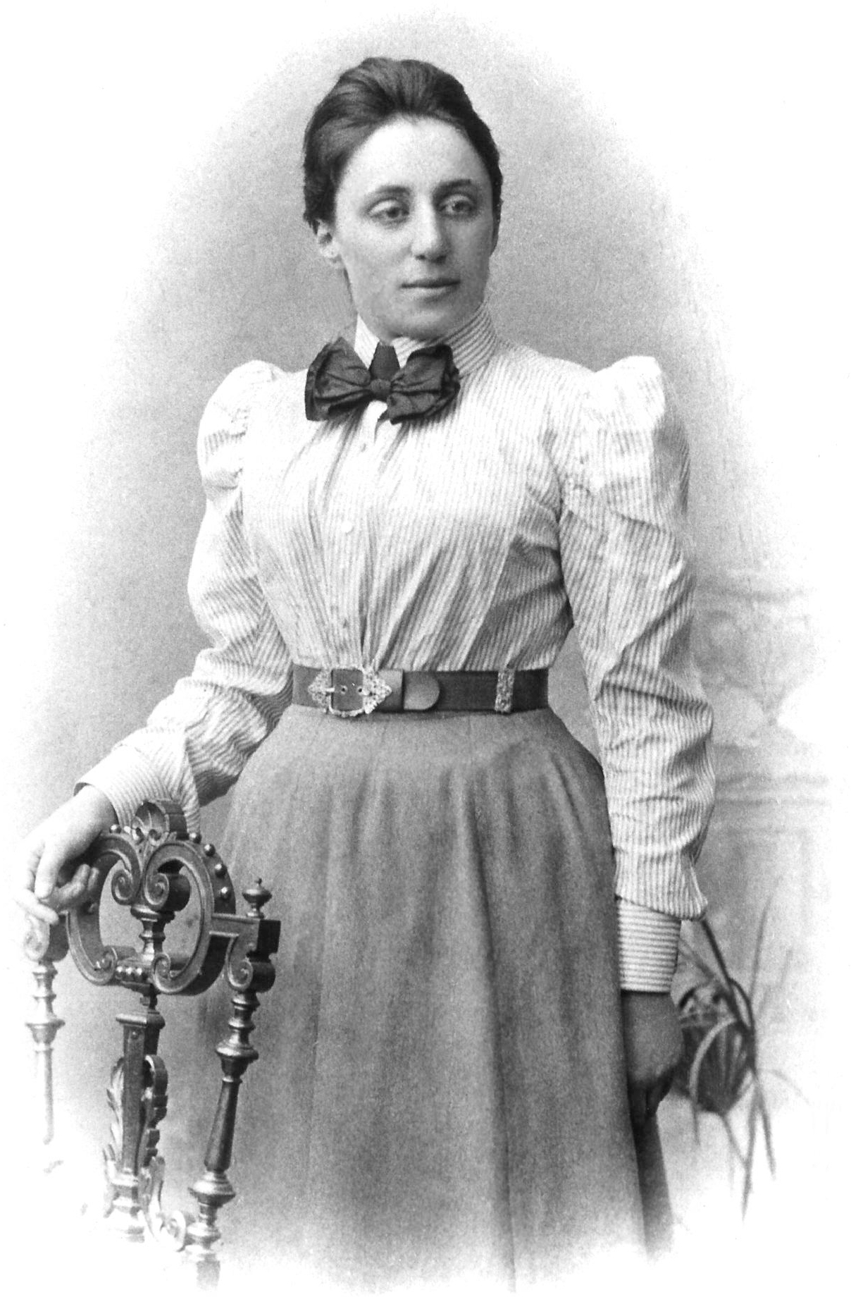
This connection was first spelled out explicitly, and proved generally, by Emmy Noether, published in 1915.  The essence of the theorem is that if the Lagrangian (which specifies the system completely) does not change when some continuous parameter is altered, then some function of the $q_i,{\dot{q}}_i$ stays the same$—$it is called a constant of the motion, an integral of the motion, or a conserved quantity.

To look further at this expression for energy, we take a closed system of particles interacting with each other, but “closed” means no interaction with the outside world (except possibly a time-independent potential).

The Lagrangian for the particles is, in Cartesian coordinates,

$L={\displaystyle \sum \frac{1}{2}{m}_i{v}_i^2-U\left({\overrightarrow{r}}_1,{\overrightarrow{r}}_2,\dots \right)}$.

A set of general coordinates $\left(q_1,\dots q_n\right)$, by definition, uniquely specifies the system configuration, so the coordinate and velocity of a particular particle $a$ are given by

$x_a=f_{x_a}\left(q_1,\dots q_n\right),{\dot{x}}_a={\displaystyle \sum _k\frac{\partial f_{x_a}}{\partial q_k}{\dot{q}}_k}.$

From this it is clear that the kinetic energy term $T={\displaystyle \sum \frac{1}{2}{m}_i{v}_i^2}$ is a homogeneous quadratic function of the $\dot{q}$ ’s (meaning every term is of degree two), so

$L=\frac{1}{2}{\displaystyle \sum _{i,k}{a}_{ik}\left(q\right){\dot{q}}_i{\dot{q}}_k}-U\left(q\right).$

This being of degree two in the time derivatives means

${\displaystyle \sum _i{\dot{q}}_i\frac{\partial L}{\partial {\dot{q}}_i}=}{\displaystyle \sum _i{\dot{q}}_i\frac{\partial T}{\partial {\dot{q}}_i}=}2T.$

(If this isn’t obvious to you, check it out with a couple of terms:  ${\dot{q}}_1^2,{\dot{q}}_1{\dot{q}}_2.$ )

Therefore for this system of interacting particles

$E={\displaystyle \sum _{i=1}^n{\dot{q}}_i\frac{\partial L}{\partial {\dot{q}}_i}}-L=2T-\left(T-U\right)=T+U.$

This expression for the energy is called the Hamiltonian:

$$H={\displaystyle \sum _{i=1}^n{p}_i{\dot{q}}_i}-L.$$

Momentum Conservation

Another conservation law follows if the Lagrangian is unchanged by displacing the whole system through a distance $\delta \overrightarrow{r}=\overrightarrow{\epsilon }.$ This means, of course, that the system cannot be in some spatially varying external field$—$it must be mechanically isolated.

It is natural to work in Cartesian coordinates to analyze this, each particle is moved the same distance ${\overrightarrow{r}}_i\to {\overrightarrow{r}}_i+\delta {\overrightarrow{r}}_i={\overrightarrow{r}}_i+\overrightarrow{\epsilon }$, so

$\delta L={\displaystyle \sum _i\frac{\partial L}{\partial {\overrightarrow{r}}_i}\cdot \delta {\overrightarrow{r}}_i=\overrightarrow{\epsilon }\cdot }{\displaystyle \sum _i\frac{\partial L}{\partial {\overrightarrow{r}}_i},}$

where the “differentiation by a vector” notation means differentiating with respect to each component, then adding the three terms. (I’m not crazy about this notation, but it’s Landau’s, so get used to it.)

For an isolated system, we must have $\delta L=0$ on displacement, moving the whole thing through empty space in any direction $\overrightarrow{\epsilon }$ changes nothing, so it must be that the vector sum ${\displaystyle \sum _i\partial L/\partial {\overrightarrow{r}}_i=0}$, so from the Cartesian Euler-Lagrange equations, writing $\dot{\overrightarrow{r}}=\overrightarrow{v},$ 

$$0={\displaystyle \sum _i\partial L/\partial {\overrightarrow{r}}_i=}{\displaystyle \sum \frac{d}{dt}}\left(\frac{\partial L}{\partial {\dot{\overrightarrow{r}}}_i}\right)={\displaystyle \sum \frac{d}{dt}}\left(\frac{\partial L}{\partial {\overrightarrow{v}}_i}\right)=\frac{d}{dt}{\displaystyle \sum \frac{\partial L}{\partial {\overrightarrow{v}}_i}},$$

and taking the system to be composed of particles of mass $m_i$ and velocity ${\overrightarrow{v}}_i$,

${\displaystyle \sum _i\frac{\partial L}{\partial {\overrightarrow{v}}_i}}={\displaystyle \sum _i{m}_i{\overrightarrow{v}}_i=\overrightarrow{P}=\text{constant,}}$

the momentum of the system.

This vector conservation law is of course three separate directional conservation laws, so even if there is an external field, if it doesn’t vary in a particular direction, the component of total momentum in that direction will be conserved.

In the Newtonian picture, conservation of momentum in a closed system follows from Newton’s third law.  In fact, the above Lagrangian analysis is really Newton’s third law in disguise. Since we’re working in Cartesian coordinates, $\partial L/\partial {\overrightarrow{r}}_i=-\partial V/\partial {\overrightarrow{r}}_i={\overrightarrow{F}}_i$, the force on the $i$ th particle, and if there are no external fields, ${\displaystyle \sum _i\partial L/\partial {\overrightarrow{r}}_i=0}$ just means that if you add all the forces on all the particles, the sum is zero.  For the Lagrangian of a two particle system to be invariant under translation through space, the potential must have the form $V\left({\overrightarrow{r}}_1-{\overrightarrow{r}}_2\right)$ , from which automatically ${\overrightarrow{F}}_{12}=-{\overrightarrow{F}}_{21}$.   

Center of Mass

If an inertial frame of reference $K^{\prime }$ is moving at constant velocity $\overrightarrow{V}$ relative to inertial frame $K,$ the velocities of individual particles in the frames are related by ${\overrightarrow{v}}_i={{\overrightarrow{v}}^{\prime }}_i+\overrightarrow{V},$ so the total momenta are related by

$\overrightarrow{P}={\displaystyle \sum _i{m}_i{\overrightarrow{v}}_i=}{\displaystyle \sum _i{m}_i{{\overrightarrow{v}}^{\prime }}_i}+\overrightarrow{V}{\displaystyle \sum _i{m}_i}={\overrightarrow{P}}^{\prime }+M\overrightarrow{V},M={\displaystyle \sum _i{m}_i.}$

If we choose $\overrightarrow{V}=\overrightarrow{P}/M,$ then ${\overrightarrow{P}}^{\prime }={\displaystyle \sum _i{m}_i{{\overrightarrow{v}}^{\prime }}_i}=0,$ the system is “at rest” in the frame $K^{\prime }.$ Of course, the individual particles might be moving, what is at rest in $K^{\prime }$ is the center of mass defined by

$M{\overrightarrow{R}}_{\text{cm}}={\displaystyle \sum _i{m}_i{\overrightarrow{r}}_i.}$

(Check this by differentiating both sides with respect to time.)

The energy of a mechanical system in its rest frame is often called its internal energy, we’ll denote it by $E_{\mathrm{int}}.$ (This includes kinetic and potential energies.)  The total energy of a moving system is then

$E=\frac{1}{2}M{\overrightarrow{V}}^2+E_{\mathrm{int}}.$

(Exercise:  Verify this.)

Angular Momentum Conservation

Conservation of momentum followed from the invariance of the Lagrangian on being displaced in arbitrary directions in space, the homogeneity of space, angular momentum conservation is the consequence of the isotropy of space$—$there is no preferred direction. 

So angular momentum of an isolated body in space is invariant even if the body is not symmetric itself. 

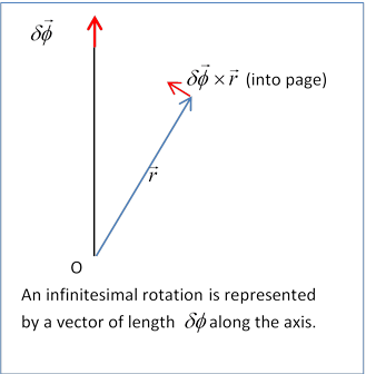
The strategy is just as before, except now instead of an infinitesimal displacement we make an infinitesimal rotation,

$\delta \overrightarrow{r}=\delta \overrightarrow{\varphi }\times \overrightarrow{r}$

and of course the velocities will also be rotated:

$\delta \overrightarrow{v}=\delta \overrightarrow{\varphi }\times \overrightarrow{v}.$

We must have

$\delta L={\displaystyle \sum _i\left(\frac{\partial L}{\partial {\overrightarrow{r}}_i}\cdot \delta {\overrightarrow{r}}_i+\frac{\partial L}{\partial {\overrightarrow{v}}_i}\cdot \delta {\overrightarrow{v}}_i\right)}=0.$

Now $\partial L/\partial {\overrightarrow{v}}_i=\partial L/\partial {\dot{\overrightarrow{r}}}_i={\overrightarrow{p}}_i$ by definition, and from Lagrange’s equations

$\partial L/\partial {\overrightarrow{r}}_i=\left(d/dt\right)\left(\partial L/\partial {\dot{\overrightarrow{r}}}_i\right)={\dot{\overrightarrow{p}}}_i,$

 so the isotropy of space implies that

${\displaystyle \sum _i\left({\dot{\overrightarrow{p}}}_i\cdot \delta \overrightarrow{\varphi }\times {\overrightarrow{r}}_i+{\overrightarrow{p}}_i\cdot \delta \overrightarrow{\varphi }\times {\overrightarrow{v}}_i\right)=0.}$

Notice the second term is identically zero anyway, since two of the three vectors in the triple product are parallel: $\left(d{\overrightarrow{r}}_i/dt\right)\times {\overrightarrow{p}}_i={\overrightarrow{v}}_i\times m{\overrightarrow{v}}_i=0$

That leaves the first term.  The equation can be written:

$\delta \overrightarrow{\varphi }\cdot \frac{d}{dt}{\displaystyle \sum _i{\overrightarrow{r}}_i\times {\overrightarrow{p}}_i}=0,$

Integrating, we find that

${\displaystyle \sum _i{\overrightarrow{r}}_i\times {\overrightarrow{p}}_i}=\overrightarrow{L}$

is a constant of motion, the angular momentum.

The angular momentum of a system is different about different origins. (Think of a single moving particle.)  The angular momentum in the rest frame is often called the intrinsic angular momentum, the angular momentum in a frame in which the center of mass is at position $\overrightarrow{R}$ and moving with velocity $\overrightarrow{V}$ is

$\overrightarrow{L}={\overrightarrow{L}}_{\text{cm frame}}+\overrightarrow{R}\times \overrightarrow{P}.$

(Exercise:  Check this.)

For a system of particles in a fixed external central field $V\left(r\right),$ the system is invariant with respect to rotations about that point, so angular momentum about that point is conserved.  For a field “cylindrically” invariant for rotations about an axis, angular momentum about that axis is conserved.

 previous  home  next  PDF