11. Introduction to Liouville’s Theorem
Michael Fowler
Paths in Simple Phase Spaces: the SHO and Falling Bodies
Let’s first think further about paths in phase space. For example, the simple harmonic oscillator, with Hamiltonian , describes circles in phase space parameterized with the variables . (A more usual notation is to write the potential term as .)
Question: are these circles the only possible paths for the oscillator to follow?
Answer: yes: any other path would intersect a circle, and at that point, with both position and velocity defined, there is only one path forward (and back) in time possible, so the intersection can’t happen.
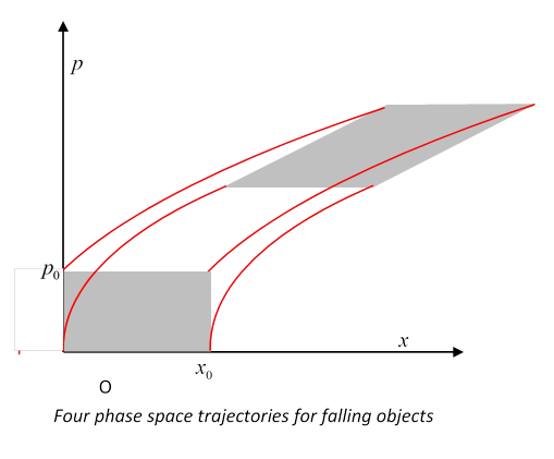 Here’s an example from Taylor of paths in phase space: four
identical falling bodies are released simultaneously, see figure, measures distance vertically down. Two are
released with zero momentum from the origin O and from a point meters down, the other two are released with
initial momenta ,
again from the points O, . (Note the difference in initial slope.)
Here’s an example from Taylor of paths in phase space: four
identical falling bodies are released simultaneously, see figure, measures distance vertically down. Two are
released with zero momentum from the origin O and from a point meters down, the other two are released with
initial momenta ,
again from the points O, . (Note the difference in initial slope.)
Check: convince yourself that all these paths are parts of parabolas centered on the -axis. (Just as the simple harmonic oscillator phase space is filled with circular paths, this one is filled with parabolas.)
Bodies released with the same initial velocity at the same time will keep the same vertical distance apart, those released with different initial velocities will keep the same velocity difference, since all accelerate at . Therefore, the area of the parallelogram formed by the four phase space points at a later time will have the same area as the initial square.
Exercise: convince yourself that all the points of an initial vertical side of the square all stay in line as time goes on, even though the line does not stay vertical.
The four sides of the square deform with time to the four sides of the parallelogram, point by point. This means that if we have a falling stone corresponding initially to a point inside the square, it will go to a point inside the parallelogram, because if somehow its path reached the boundary, we would have two paths in phase space intersecting, and a particle at one point in phase space has a uniquely defined future path (and past).
Following Many Systems: a “Gas” in Phase Space
We’ve looked at four paths in phase space, corresponding to four falling bodies, all beginning at , but with different initial co-ordinates in . Suppose now we have many falling bodies, so that at a region of phase space can be imagined as filled with a “gas” of points, each representing one falling body, initially at
The argument above about the phase space path of a point within the square at staying inside the square as time goes on and the square distorts to a parallelogram must also be true for any dynamical system, and any closed volume in phase space, since it depends on phase space paths never intersecting: that is,
if at t = 0 some closed surface in phase space contains a number of points of the gas, those same points remain inside the surface as it develops in time -- none exit or enter.
For the number of points sufficiently large, the phase space time development looks like the flow of a fluid.
Liouville’s Theorem: Local Gas Density Is Constant along a Phase Space Path
The falling bodies phase space square has one more lesson for us: visualize now a uniformly dense gas of points inside the initial square. Not only does the gas stay within the distorting square, the area it covers in phase space remains constant, as discussed above, so the local gas density stays constant as the gas flows through phase space.
Liouville’s theorem is that this constancy of local density is true for general dynamical systems.
Landau’s Proof Using the Jacobian
Landau gives a very elegant proof of elemental volume invariance under a general canonical transformation, proving the Jacobian multiplicative factor is always unity, by clever use of the generating function of the canonical transformation.
Jacobians have wide applicability in different areas of physics, so this is a good time to review their basic properties, which we do below, as a preliminary to giving the proof.
It must be admitted that there are simpler ways of deriving Liouville’s theorem, directly from Hamilton’s equations, the reader may prefer to skip the Jacobian proof at first reading.
Jacobian for Time Evolution
As we’ve established, time development is equivalent to a canonical coordinate transformation,
.
Since we already know that the number of points inside a closed volume is constant in time, Liouville’s theorem is proved if we can show that the volume enclosed by the closed surface is constant, that is, with denoting the volume evolves to become, we must prove
If you’re familiar with Jacobians, you know that (by definition)
where the Jacobian
Liouville’s theorem is therefore proved if we can establish that If you’re not familiar with Jacobians, or need reminding, read the next section!
Jacobians 101
You can skip this section if you're already familiar with Jacobians.
Suppose we are integrating a function over some region of ordinary three-dimensional space,
but we want to change variables of integration to a different set of coordinates such as, for example, . The new coordinates are of course functions of the original ones , etc., and we assume that in the region of integration they are smooth, well-behaved functions. We can’t simply re-express in terms of the new variables, and replace the volume differential by , that gives the wrong answerin a plane, you can’t replace with , you have to use . That extra factor is called the Jacobian, it’s clear that in the plane a small element with sides of fixed lengths is bigger the further it is from the origin, not all elements are equal, so to speak. Our task is to construct the Jacobian for a general change of coordinates.
We need to think carefully about the volumes in the three-dimensional space represented by and by . Of course, the ’s are just ordinary perpendicular Cartesian axes so the volume is just the product of the three sides of the little box, . Imagine this little box, its corner closest to the origin at and its furthest point at the other end of the body diagonal at Let’s take these two points in the coordinates to be at and . In visualizing this, bear in mind that the axes need not be perpendicular to each other (but they cannot all lie in a plane, that would not be well-behaved).
For the coordinate integration, we imagine filling the space with little cubical boxes. For the integration, we have a system of space filling infinitesimal parallelepipeds, in general pointing different ways in different regions (think ). What we need to find is the volume of the incremental parallelepiped with sides we’ll write as vectors in -coordinates, . These three incremental vectors are along the corresponding coordinate axes, and the three added together are the displacement from to .
Hence, in components,
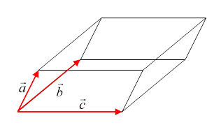 Now the volume of the parallelepiped with sides the three
vectors from the origin is (recall is the area of the parallelogram, then the dot
product singles out the component of perpendicular to the plane of ).
Now the volume of the parallelepiped with sides the three
vectors from the origin is (recall is the area of the parallelogram, then the dot
product singles out the component of perpendicular to the plane of ).
So, the volume corresponding to the increments in space is
writing (Landau’s notation) for the determinant, which is in fact the Jacobian, often denoted by .
The standard notation for this determinantal Jacobian is
So the appropriate replacement for the three dimensional incremental volume element represented in the integral by is
The inverse
this is easily established using the chain rule for differentiation.
Exercise: check this!
Thus the change of variables in an integral is accomplished by rewriting the integrand in the new variables, and replacing
The argument in higher dimensions is just the same: on going to dimension , the hypervolume element is equal to that of the dimensional element multiplied by the component of the new vector perpendicular to the dimensional element. The determinantal form does this automatically, since a determinant with two identical rows is zero, so in adding a new vector only the component perpendicular to all the earlier vectors contributes.
We’ve seen that the chain rule for differentiation gives the inverse as just the Jacobian with numerator and denominator reversed, it also readily yields
and this extends trivially to dimensions.
It’s also evident form the determinantal form of the Jacobian that
,
identical variables in numerator and denominator can be canceled. Again, this extends easily to dimensions.
Jacobian proof of Liouville’s Theorem
After this rather long detour into Jacobian theory, recall we are trying to establish that the volume of a region in phase space is unaffected by a canonical transformation, we need to prove that
,
and that means we need to show that the Jacobian
Using the theorems above about the inverse of a Jacobian and the chain rule product,
Now invoking the rule that if the same variables appear in both numerator and denominator, they can be cancelled,
Up to this point, the equations are valid for any nonsingular transformationbut to prove the numerator and denominator are equal in this expression requires that the equation be canonical, that is, be given by a generating function, as explained earlier.
Recall now the properties of the generating function ,
from which
.
In the expression for the Jacobian , the element of the numerator is
In terms of the generating function this element is
Exactly the same procedure for the denominator gives the element to be
In other words, the two determinants are the same (rows and columns are switched, but that doesn’t affect the value of a determinant). This means and Liouville’s theorem is proved.
Simpler Proof of Liouville’s Theorem
Landau’s proof given above is extremely elegant: since phase space paths cannot intersect, point inside a volume stay inside, no matter how the volume contorts, and since time development is a canonical transformation, the total volume, given by integrating over volume elements , stays the same, since it’s an integral over the corresponding volume elements and we’ve just shown that .
 Here we’ll take a slightly different point of view: we’ll
look at a small square in phase space and track how its edges are moving, to
prove its volume isn’t changing. (We’ll stick to one dimension, but the
generalization is straightforward.)
Here we’ll take a slightly different point of view: we’ll
look at a small square in phase space and track how its edges are moving, to
prove its volume isn’t changing. (We’ll stick to one dimension, but the
generalization is straightforward.)
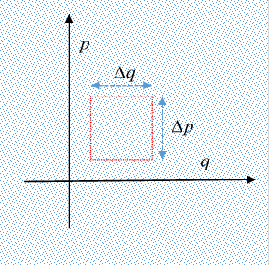
The points here represent a “gas” of many systems in the two dimensional phase space, and with a small square area , tagged by having all the systems on its boundary represented by dots of a different color. What is the incremental change in area of this initially square piece of phase space in time ?
Begin with the top edge: the particles are all moving with velocities , but of course the only change in area comes from the term, that’s the outward movement of the boundary, so the area change in from the movement of this boundary will be . Meanwhile, there will be a similar term from the bottom edge, and the net contribution, top plus bottom edges, will depend on the change in from bottom to top, that is, a net area change from movement of these edges .
Adding in the other two edges (the sides), with an exactly similar argument, the total area change is
.
But from Hamilton’s equations , so
and therefore
establishing that the total incremental area change as the square distorts is zero.
The conclusion is that the flow of the gas of systems in phase space is like an incompressible fluid, but with one important qualification: the density may vary with position! It just doesn’t vary along a dynamical path.
Energy Gradient and Phase Space Velocity
For a time-independent Hamiltonian, the path in phase space is a constant energy line, and we can think of the whole phase space as delineated by many such lines, exactly analogous to contour lines joining points at the same level on a map of uneven terrain, energy corresponding to height above sea level. The gradient at any point, the vector pointing exactly uphill and therefore perpendicular to the constant energy path, is
,
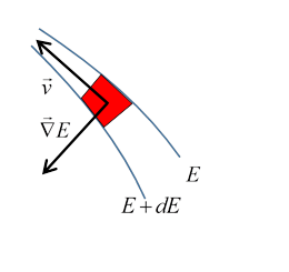 here .
The velocity of a system’s point moving through phase space is
here .
The velocity of a system’s point moving through phase space is
.
This vector is perpendicular to the gradient vector, as it must be, of course, since the system moves along a constant energy path. But, interestingly, it has the same magnitude as the gradient vector! What is the significance of that? Imagine a small square sandwiched between two phase space paths close together in energy, and suppose the distance between the two paths is decreasing, so the square is getting squeezed, at a rate equal to the rate of change of the energy gradient. But at the same time it must be getting stretched along the direction of the path, an amount equal to the rate of change of phase space velocity along the pathand they are equal. So, this is just Liouville again, its area doesn’t change.