13. Adiabatic Invariants and Action-Angle Variables
Michael Fowler
Adiabatic Invariants
Imagine a particle in one dimension oscillating back and forth in some potential. The potential doesn’t have to be harmonic, but it must be such as to trap the particle, which is executing periodic motion with period . Now suppose we gradually change the potential, but keeping the particle trapped. That is, the potential depends on some parameter , which we change gradually, meaning over a time much greater than the time of oscillation:
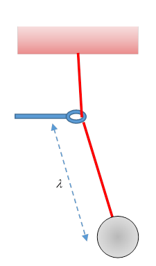
A crude demonstration is a simple pendulum with a string of variable length, for example (see figure) one hanging from a fixed support, but the string passing through a small loop that can be moved vertically to change the effective length.
If were fixed, the system would have constant energy and period As is gradually changed from outside, there will be energy exchange in general, we’ll write the Hamiltonian the energy of the system will be (Of course, also depends on the initial energy before the variation began.) Remember now that from Hamilton’s equations so during the variation
It’s clear from the diagram that the energy fed into the system as the ring moves slowly down varies throughout the cycle—for example, when the pendulum is close to vertically down, its energy will be almost unaffected by moving the ring.
Moving slowly down means varies very little in one cycle of the system, we can average over a cycle:
where
Now Hamilton’s equation means that we can replace with , so the time for going round one complete cycle is
(This won’t integrate to zero, because on the return leg both and will be negative.)
Therefore, replacing in as well,
Now, we assume are varying slowly enough that they are close to constant over one cycle, meaning that at a given point on the circuit, the momentum can be written , regarding as constant and independent parameters. (We can always adjust at fixed by giving the pendulum a little push!)
If we now partially differentiate with respect to keeping constant (appropriate infinitesimal pushes required!), we get, at point on the circuit,
which is the integrand in the numerator of our expression for , so
In the denominator, we’ve replaced by
Rearranging,
This can be written
is an adiabatic invariant: That means it stays constant when the parameters of the system change gradually, even though the system’s energy changes.
Important! The partial derivative with respect to energy determines the period of the motion:
(Note: here is another connection with quantum mechanics. If the system is connected to the outside world, for example if the orbiting particle is charged, as it usually is, and can therefore emit radiation, since in quantum mechanics successive action numbers differ by integers, and the quantum of action is , the energy radiated per quantum drop in action is . This is of course in the classical limit of high quantum numbers.)
Notice that is the area of phase space enclosed by the integral,
For the SHO, it’s easy to check from the area of the ellipse that :
Take
The phase space elliptical orbit has semi-axes with lengths , so the area enclosed is
The bottom line is that as we gradually change the spring strength (or, for that matter, the mass) of an oscillator (not necessarily harmonic), the energy changes proportionally with the frequency.
Adiabatic Invariance and Quantum Mechanics
This finding, the invariance of for slow variation of the potential strength in a simple harmonic oscillator, connects directly with quantum mechanics, as was first pointed out be Einstein in 1911. Suppose the (quantum mechanical) oscillator is in the energy eigenstate with Then the spatial wave function has zeros. If the potential is changed slowly enough (meaning little change over one cycle of oscillation) the oscillator will not jump to another eigenstate (or, more precisely, the probability will go to zero with the speed of change). The wave function will gradually stretch (or compress) but the number of zeroes will not change. Therefore the energy will stay at and track with Of course, the classical system is a little different: the quantum system is “locked in” to a particular state if the perturbation has vanishingly small frequency components corresponding to the energy differences to available states. The classical system, on the other hand, can move to states arbitrarily close in energy. Landau gives a nontrivial analysis of the classical system, concluding that the change in the adiabatic “invariant” is of order for an external change acting over a time
Action-Angle Variables
For a closed one-dimensional system undergoing finite motion (essentially a bound state), the equations of motion can be reformulated using the action variable in place of the energy is a function of energy alone in a closed one-dimensional system, and vice versa.
We’re visualizing here a particle moving back and forth in a one-dimensional well with potential zero at the origin, and the potential never decreasing on going out from the origin to infinity. Obviously, if a potential has two low points, local bound states can arise in different places, and the relationship is complicated, with different branches, possibly coming together at high energies.
Important! Notice the integral sign in the expression for the action variable is signifying an integral around a closed path, a circuit. Don’t confuse this integral with the abbreviated action integral, which has the same integrand, but is an integral along a contour from a fixed starting point, say the origin, to the endpoint , not going around a closed path. (Apologies for using the same letter for the differential and the endpoint, just following Landau.)
In the spirit of the discussion of constants of motion above, we make a canonical transformation to as the new “momentum”, using as generating function the abbreviated action
The original momentum
The new “coordinate” conjugate to the momentum will be
This is called an angle variable, is the action variable, they are canonical.
To find Hamilton’s equations in the transformed variables, since there is no time-dependence in the transformation, and the system is closed, the energy remains constant. Also, the energy is a function of (meaning not of )
Hence
so the angle is a linear function of time:
One further point about the action variable and the action: since we define the action as
it follows that if we track the change in this integral as time goes on and the system moves round and round the circuit in phase space, an additional term will be added to the action for each time round, so the action is multi-valued.
*Kepler Orbit Action-Angle Variables
We have not yet covered Kepler orbits, so skip this section for now: it's here to refer back to later. It's from Landau, p 167.
For motion confined to a plane, we can take the central potential analysis with and , the angular momentum, so the Hamiltonian is
The Hamilton-Jacobi equation is therefore
So, following the previous analysis of separation of variables for motion in a central potential, here
The action variable for the angular motion is just the angular momentum itself,
And the radial action variable, with potential , is
(Details on doing the integral are given in the Appendix, Mathematica can do it too.)
So the energy is
The motion is degenerate: the two fundamental frequencies coincide,
This has major consequences in quantum mechanics: the actions are all quantized in units of Planck's constant, for the hydrogen atom, from the formula above, the energy depends only on the sum of the quantum numbers: above the ground state, energy levels are degenerate, which is why the energy spectrum has the deceptively simple form so successfully explained by the Bohr model.
The orbital parameters, semi-latus rectum and eccentricity, from and , are
Recall the semi-major axis is given by and from the above expression
in the hydrogen atom quantum number notation.
Appendix: Doing the Integral for The Radial Action Ir
The integral can be put in the form
which can be integrated by taking a contour encircling the cut from to The integral will have a contribution from the pole at the origin equal to , and another from the circle at infinity, which is
.
Equating coefficients (multiplying the term inside the square root by )
So the contribution from the origin gives the the circle at infinity .