8. A New Way to Write the Action Integral
Michael Fowler
Introduction
Following Landau, we'll first find how the action integral responds to incremental changes in the endpoint coordinates and times, then use the result to write the action integral itself in a new, more intuitive way. This new formulation shows very directly the link to quantum mechanics, and variation of the action in this form gives Hamilton's equations immediately.
Function of Endpoint Position
We’ll now think of varying the action in a slightly different way. (Note: We’re using Landau's notation.) Previously, we considered the integral of the Lagrangian over all possible different paths from the initial place and time to the final place and time and found the path of minimum action. Now, though, we’ll start with that path, the actual physical path, and investigate the corresponding action as a function of the final endpoint variables, given a fixed beginning place and time.
Taking one degree of freedom (the generalization is straightforward), for a small path variation the incremental change in action
(Recall that first term comes from the calculus of variations when we allow the end point to vary—it’s exactly the same point we previously discussed in the brachistochrone problem of fastest time for a given horizontal distance, allowing the vertical position of the endpoint to be a free parameter.)
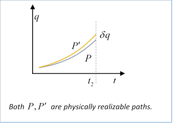
With the incremental variation, we’ve gone from the physical path (followed by the system in configuration space from to ) to a second path beginning at the same place and time, and ending at the same time as but at a slightly different place .
Both paths are fully determined by their initial and final positions and times, so must correspond to slightly different initial velocities. The important point is that since both paths describe the natural dynamical development of the system from the initial conditions, the system obeys the equations of motion at all times along both paths, and therefore the integral term in the above equation is identically zero.
Writing the action, regarded as a function of the final position variable, with the final time fixed at , has the differential
For the multidimensional case, the incremental change in the action on varying the final position variable is given by (dropping the superscript)
Function of Endpoint Time
What about the action as a function of the final point arrival time?
Since the total time derivative the value of the Lagrangian at the endpoint. Remember we are defining the action at a point as that from integrating along the true path up to that point.
Landau denotes by just , so he writes , and we’ll be doing this, but it’s crucial to keep in mind that the endpoint position and time are the variables here!
If we now allow an incremental time increase, , with the final coordinate position as a free parameter, the dynamical path will now continue on, to an incrementally different finishing point.
This will give (with understood from now on to mean , and means )
Putting this together with gives immediately the partial time derivative
and therefore, combining this with the result from the previous section,
This, then, is the total differential of the action as a function of the spatial and time coordinates of the end of the path.
Varying Both Ends
The argument given above for the incremental change in action from varying the endpoint is clearly equally valid for varying the beginning point of the integral (there will be a sign change, of course), so
The initial and final coordinates and times specify the action and the time development of the system uniquely.
(Note: We’ll find this equation again in the section on canonical transformations—the action will be seen there to be the generating function of the time-development canonical transformation, this will become clear when we get to it.)
Another Way of Writing the Action Integral
Up to this point, we’ve always written the action as an integral of the Lagrangian with respect to time along the path,
.
However, the expression derived in the last section for the increment of action generated by an incremental change in the path endpoint is clearly equally valid for the contribution to the action from some interior increment of the path, say from to , so we can write the total action integral as the sum of these increments:
In this integral, of course, the add up to cover the whole path.
(In writing we’re following Landau’s default practice of taking the action as a function of the final endpoint coordinates and time, assuming the beginning point to be fixed. This is almost always finewe’ll make clear when it isn’t.)
How this Classical Action Relates to Phase in Quantum Mechanics
The link between classical and quantum mechanics is particularly evident in the expression for the action integral given above. In the so-called semi-classical regime of quantum mechanics, the de Broglie waves oscillate with wavelengths much smaller than typical sizes in the system. This means that locally it’s an adequate approximation to treat the Schrödinger wave function as a plane wave,
where the amplitude function only varies over distances much greater than the wavelength, and times far longer than the oscillation period. This expression is valid in almost all the classically accessible regions, invalid in the neighborhood of turning points, but the size of those neighborhoods goes to zero in the classical limit.
As we’ve discussed earlier, in the Dirac-Feynman formulation of quantum mechanics, to find the probability amplitude of a particle propagating from one point to another, we add contributions from all possible paths between the two points, each path contributing a term with phase equal to times the action integral along the path.
From the semi-classical Schrödinger wave function above, it’s clear that the change in phase from a small change in the endpoint is , coinciding exactly with the incremental contribution to the action in
So again we see, here very directly, how the action along a classical path is a multiple of the quantum mechanical phase change along the path.
Hamilton’s Equations from Action Minimization
For arbitrary small path variations in phase space, the minimum action condition using the form of action given above generates Hamilton’s equations.
(Note for nitpickers: This may seem a bit surprising, since we generated this form of the action using the equations along the actual dynamical path, how can we vary it and still use them? Bear with me, you’ll see.)
We’ll prove this for a one dimensional system, it’s trivial to go to many variables, but it clutters up the equations.
For a small path deviation , the change in the action is
and integrating by parts, with at the endpoints,
The path variations are independent and arbitrary, so must have identically zero coefficientsHamilton’s equations follow immediately,
Again, it’s worth emphasizing the close parallel with quantum mechanics: Hamilton’s equations written using Poisson brackets are:
In quantum mechanics, the corresponding Heisenberg equations of motion for position and momentum operators in terms of commutators are
How Can p, q Really Be Independent Variables?
It may seem a little odd at first that varying as independent variables leads to the same equations as the Lagrangian minimization, where we only varied and that variation “locked in” the variation of And, isn’t defined in terms of by which is some function of ? So wouldn’t varying automatically determine the variation of ?
The answer is, no, is not defined as from the start in Hamilton’s formulation. In this Hamiltonian approach, really are taken as independent variables, then varying them to find the minimum path gives the equations of motion, including the relation between and .
This comes about as follows: Along the minimum action path, we just established that
We also have that so (Legendre transformation!)
from which, along the physical path, So this identity, previously written as the definition of now arises as a consequence of the action minimization in phase space.