previous  home  next  PDF

15. Keplerian Orbits

Michael Fowler

Preliminary: Polar Equations for Conic Section Curves

As we shall find, Newton’s equations for particle motion in an inverse-square central force give orbits that are conic section curves.  Properties of these curves are fully discussed in the accompanying “Math for Orbits” lecture, here for convenience we give the relevant polar equations for the various possibilities.

For an ellipse, with eccentricity $e$ and semilatus rectum (perpendicular distance from focus to curve) $\ell :$ 

$$\frac{\ell }{r}=1+e\cos \theta .$$

Recall the eccentricity $e$ is defined by the distance from the center of the ellipse to the focus being $ae,$ where $a$ is the semi-major axis, and $\ell =a\left(1-e^2\right)=b^2/a.$  

For a parabola,

$\ell =r\left(1+\cos \theta \right).$

For a hyperbolic orbit with an attractive inverse square force, the polar equation with origin at the center of attraction is

$$\frac{\ell }{r}=1-e\cos \theta$$

where ${\theta }_{\text{asymptote}}<\theta <2\pi -{\theta }_{\text{asymptote}}.$ (Of course, the physical path of the planet (say) is only one branch of the hyperbola.)

The $\left(r,\theta \right)$ origin is at the center of attraction (the Sun), geometrically this is one focus of the hyperbola, and for this attractive case it’s the focus “inside” the curve.

For a hyperbolic orbit with a repulsive inverse square force (such as Rutherford scattering), the origin is the focus “outside” the curve, and to the right (in the usual representation):

$$\frac{\ell }{r}=-e\cos \theta -1,$$

with angular range $-{\theta }_{\text{asymptote}}<\theta <{\theta }_{\text{asymptote}}.$ 

Summary

We’ll begin by stating Kepler’s laws, then apply Newton’s Second Law to motion in a central force field.  Writing the equations vectorially leads easily to the conservation laws for angular momentum and energy.  

Next, we use Bernoulli’s change of variable $u=1/r$ to prove that the inverse-square law gives conic section orbits.

A further vectorial investigation of the equations, following Hamilton, leads naturally to an unsuspected third conserved quantity, after energy and angular momentum, the Runge Lenz vector.

Finally, we discuss the rather surprising behavior of the momentum vector as a function of time. 

Kepler’s Statement of his Three Laws

1. The planets all move in elliptical orbits with the Sun at one focus.

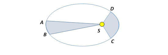
2. As a planet moves in its orbit, the line from the center of the Sun to the center of the planet sweeps out equal areas in equal times, so if the area SAB (with curved side AB) equals the area SCD, the planet takes the same time to move from A to B as it does from C to D. 

My applet illustrating this is here!.

3. The time it takes a planet to make one complete orbit around the sun $T$ (one planet year) is related to the length of the semimajor axis of the ellipse $a$:

$T^2\propto a^3.$

In other words, if a table is made of the length of year $T$ for each planet in the Solar System, and the length of the semimajor axis of the ellipse $a$, and $T^2/a^3$ is computed for each planet, the numbers are all the same.

These laws of Kepler’s are precise (apart from tiny relativistic corrections, undetectable until centuries later) but they are only descriptive$—$Kepler did not understand why the planets should behave in this way.  Newton’s great achievement was to prove that all this complicated behavior followed from one simple law of attraction.

Dynamics of Motion in a Central Potential: Deriving Kepler’s Laws

Conserved Quantities

The equation of motion is:

$m\ddot{\overrightarrow{r}}=-f\left(r\right)\widehat{\overrightarrow{r}}$.

Here we use the hat ^ to denote a unit vector, so $f\left(r\right)$ gives the magnitude (and sign) of the force.  For Kepler’s problem, $f\left(r\right)=GMm/r^2$.

(Strictly speaking, we should be using the reduced mass for planetary motion, for our Solar System, that is a small correction.  It can be put in at the end if needed.)

Let’s see how using vector methods we can easily find constants of motion:  first, angular momentum$—$just act on the equation of motion with $\overrightarrow{r}\times :$

$m\overrightarrow{r}\times \ddot{\overrightarrow{r}}=-f\left(r\right)\overrightarrow{r}\times \widehat{\overrightarrow{r}}$

Since $\overrightarrow{r}\times \widehat{\overrightarrow{r}}=0$, we have $\overrightarrow{r}\times m\ddot{\overrightarrow{r}}=0$, which immediately integrates to

$\overrightarrow{r}\times m\dot{\overrightarrow{r}}=\overrightarrow{L}$,

 a constant, the angular momentum, and note that $\overrightarrow{L}\cdot \overrightarrow{r}=0=\overrightarrow{L}\cdot \dot{\overrightarrow{r}},$ so the motion will always stay in a  plane, with $\overrightarrow{L}$ perpendicular to the plane.

This establishes that motion in a purely central force obeys a conservation law: that of angular momentum.

 (As we've discussed earlier in the course, conserved quantities in dynamical systems are always related to some underlying symmetry of the Hamiltonian. The conservation of angular momentum comes from the spherical symmetry of the system: the attraction depends only on distance, not angle.  In quantum mechanics, the angular momentum operator is a rotation operator:  the three components of the angular momentum vector are conserved, are constants of the motion, because the Hamiltonian is invariant under rotation.  That is, the angular momentum operators commute with the Hamiltonian.  The classical analogy is that they have zero Poisson brackets with the Hamiltonian.)

To get back to Kepler’s statement of his Laws, notice that when the planet moves through an incremental distance $d\overrightarrow{r}$ it “sweeps out” an area $\frac{1}{2}\overrightarrow{r}\times d\overrightarrow{r}$, so the rate of sweeping out area is $dA/dt=\frac{1}{2}\left|\overrightarrow{r}\times \dot{\overrightarrow{r}}\right|=L/2m.$  Kepler’s Second Law is just conservation of angular momentum!

Second, conservation of energy: this time, we act on the equation of motion with $\dot{\overrightarrow{r}}\cdot$ :

$m\dot{\overrightarrow{r}}\cdot \ddot{\overrightarrow{r}}=-f\left(r\right)\widehat{\overrightarrow{r}}\cdot \dot{\overrightarrow{r}}.$

This immediately integrates to

$\frac{1}{2}m{\dot{\overrightarrow{r}}}^2-{\displaystyle \underset{r}{\overset{\infty }{\int }}f\left(r\right)dr=E}.$

 Another conservation law coming from a simple integral: conservation of energy.  What symmetry does that correspond to? The answer is the invariance of the Hamiltonian under time: the central force is time invariant, and we’re assuming there are time-dependent potential terms, (such as from another star passing close by).

 Standard Calculus Derivation of Kepler’s First Law

The first mathematical proof that an elliptic orbit about a focus meant an inverse-square attraction was given by Newton, using Euclidean geometry (even though he invented calculus!).  The proof is notoriously difficult to follow.  Bernoulli found a fairly straightforward calculus proof in polar coordinates by changing the variable to $u=1/r.$  

The first task is to express $\overrightarrow{F}=m\overrightarrow{a}$ in polar, meaning $\left(r,\theta \right),$ coordinates. 

The simplest way to find the expression for acceleration is to parameterize the planar motion as a complex number:  position $r{e}^{i\theta }$, velocity $\dot{r}{e}^{i\theta }+ir\dot{\theta }{e}^{i\theta }$, notice this means $\left(\dot{r},r\dot{\theta }\right)$ since the $i$ ensures the $r\dot{\theta }$ term is in the positive $\theta$ direction, and differentiating again gives

$\overrightarrow{a}=\ddot{\overrightarrow{r}}=\left(\ddot{r}-r{\dot{\theta }}^2,r\ddot{\theta }+2\dot{r}\dot{\theta }\right).$

For a central force, the only acceleration is in the $r$ direction, so $r\ddot{\theta }+2\dot{r}\dot{\theta }=0,$ which integrates to give

$m{r}^2\dot{\theta }=L,$

the constancy of angular momentum.

Equating the radial components,

$$\frac{d^{2}r}{d{t}^2}-r{\dot{\theta }}^2=-\frac{GM}{r^2}$$

This isn’t ready to integrate yet, because $\dot{\theta }$ varies too.  But since the angular momentum $L=m{r}^2\dot{\theta }$ is constant, we can eliminate $\dot{\theta }$ from the equation, giving:

$$\begin{array}{c}\frac{d^{2}r}{d{t}^2}=-\frac{GM}{r^2}+r{\left(\frac{L}{m{r}^2}\right)}^2\\ =-\frac{GM}{r^2}+\frac{L^2}{m^2{r}^3}\end{array}$$

This doesn’t look too promising, but Bernoulli came up with two clever tricks. The first was to change from the variable $r$ to its inverse, $u=1/r$. The other was to use the constancy of angular momentum to change the variable $t$ to $\theta$.

 Putting these together:

$$L=m{r}^2\dot{\theta }=\frac{m}{u^2}\frac{d\theta }{dt}$$

so

$$\frac{d}{dt}=\frac{L{u}^2}{m}\frac{d}{d\theta }.$$

Therefore

$$\frac{dr}{dt}=\frac{d}{dt}\left(\frac{1}{u}\right)=-\frac{1}{u^2}\frac{du}{dt}=-\frac{L}{m}\frac{du}{d\theta }$$

and similarly

$$\frac{d^{2}r}{d{t}^2}=-\frac{L^2{u}^2}{m^2}\frac{d^{2}u}{d{\theta }^2}.$$

Going from $r$ to $u$ in the equation of motion

$$\frac{d^{2}r}{d{t}^2}=-\frac{GM}{r^2}+\frac{L^2}{m^2{r}^3}$$

we get

$$-\frac{L^2{u}^2}{m^2}\frac{d^{2}u}{d{\theta }^2}=-GM{u}^2+\frac{L^2{u}^3}{m^2},$$

or

$$\frac{d^{2}u}{d{\theta }^2}+u=\frac{GM{m}^2}{L^2}.$$

This equation is easy to solve!  The solution is

$$u=\frac{1}{r}=\frac{GM{m}^2}{L^2}+C\cos \theta$$

where $C$ is a constant of integration, determined by the initial conditions.

This proves that Kepler’s First Law follows from the inverse-square nature of the force, because (see beginning of lecture) the equation above is exactly the standard $\left(r,\theta \right)$ equation of an ellipse of semi major axis $a$ and eccentricity $e$, with the origin at one focus:

$$\frac{a\left(1-e^2\right)}{r}=1+e\cos \theta .$$

Comparing the two equations, we can find the geometry of the ellipse in terms of the angular momentum, the gravitational attraction, and the initial conditions. The angular momentum is

$L^2=GM{m}^{2}a\left(1-e^2\right)=GM{m}^2{b}^2/a.$

A Vectorial Approach:  Hamilton’s Equation and the Runge Lenz Vector

(Mainly following Milne, Vectorial Mechanics, p 235 on.)

Laplace and Hamilton developed a rather different approach to this inverse-square orbit problem, best expressed vectorially, and made a surprising discovery: even though conservation of angular momentum and of energy were enough to determine the motion completely, for the special case of an inverse-square central force, something else was conserved.  So the system has another symmetry!

Hamilton’s approach (actually vectorized by Gibbs) was to apply the operator $\overrightarrow{L}\times$ to the equation of motion $m\ddot{\overrightarrow{r}}=-f\left(r\right)\widehat{\overrightarrow{r}}$:

$\overrightarrow{L}\times m\ddot{\overrightarrow{r}}=-f\left(r\right)\left[\left(\overrightarrow{r}\times m\dot{\overrightarrow{r}}\right)\times \widehat{\overrightarrow{r}}\right]$

Now

$$\left(\overrightarrow{r}\times \dot{\overrightarrow{r}}\right)\times \widehat{\overrightarrow{r}}=-\overrightarrow{r}\left(\widehat{\overrightarrow{r}}\cdot \dot{\overrightarrow{r}}\right)+r\dot{\overrightarrow{r}}=r^2\left(\frac{\dot{\overrightarrow{r}}}{r}-\frac{\overrightarrow{r}}{r^2}\frac{dr}{dt}\right)=r^2\frac{d}{dt}\left(\frac{\overrightarrow{r}}{r}\right)=r^2\frac{d\widehat{\overrightarrow{r}}}{dt},$$

so

$$\overrightarrow{L}\times m\ddot{\overrightarrow{r}}=-m{r}^{2}f\left(r\right)\frac{d\widehat{\overrightarrow{r}}}{dt}.$$

This is known as Hamilton’s equation.

In fact, it's pretty easy to understand on looking it over: $d\widehat{\overrightarrow{r}}/dt$ has magnitude $\dot{\theta }$ and direction perpendicular to $\overrightarrow{r},$ $m\ddot{\overrightarrow{r}}=-f\left(r\right)\widehat{\overrightarrow{r}}$,  $m{r}^2\dot{\theta }=L$, etc.

It isn’t very useful, though$—$except in one case, the inverse-square: $f\left(r\right)=k/r^2$  (so $k=GM.$ ) 

Then it becomes tractable:  $\overrightarrow{L}\times m\ddot{\overrightarrow{r}}=-m{r}^{2}f\left(r\right)\frac{d\widehat{\overrightarrow{r}}}{dt}=-km\frac{d\widehat{\overrightarrow{r}}}{dt}$,  and$—$surprise$—$this integrates immediately to

$\overrightarrow{L}\times m\dot{\overrightarrow{r}}=-km\widehat{\overrightarrow{r}}-\overrightarrow{A}$

where $\overrightarrow{A}$ is a vector constant of integration,  that is to say we find

$\overrightarrow{A}=\overrightarrow{p}\times \overrightarrow{L}-km\widehat{\overrightarrow{r}}$

is constant throughout the motion! 

This is unexpected:  we found the usual conserved quantities, energy and angular momentum, and indeed they were sufficient for us to find the orbit.  But for the special case of the inverse-square law, something else is conserved.   It’s called the Runge Lenz vector (sometimes Laplace Runge Lenz, and in fact Runge and Lenz don’t really deserve the fame—they just rehashed Gibbs’ work in a textbook). 

From our earlier discussion, this conserved vector must correspond to a symmetry.  Finding the orbit gives some insight into what’s special about the inverse-square law.

Deriving the Orbital Equation from the Runge-Lenz Vector

The Runge Lenz vector gives a very quick derivation of the elliptic orbit, without Bernoulli’s unobvious tricks in the standard derivation presented above.

First, taking the dot product of $\overrightarrow{A}=\overrightarrow{p}\times \overrightarrow{L}-km\widehat{\overrightarrow{r}}$ with the angular momentum $\overrightarrow{L}$, we find $\overrightarrow{A}\cdot \overrightarrow{L}=km\widehat{\overrightarrow{r}}\cdot \overrightarrow{L}=0$, meaning that the constant vector $\overrightarrow{A}$ lies in the plane of the orbit.

Next take the dot product of $\overrightarrow{A}$ with $\overrightarrow{r}$, and since $\overrightarrow{p}\times \overrightarrow{L}\cdot \overrightarrow{r}=\overrightarrow{L}\cdot \overrightarrow{r}\times \overrightarrow{p}=L^2$, we find $L^2=kmr+\overrightarrow{A}\cdot \overrightarrow{r}$, or

$$\frac{\ell }{r}=1+e\cos \theta$$

where $\ell =L^2/km,e=A/km$ and θ  is the angle between the planet’s orbital position and the Runge Lenz vector $\overrightarrow{A}$.

This is the standard $\left(r,\theta \right)$ equation for an ellipse, with $\ell$ the semi-latus rectum (the perpendicular distance from a focus to the ellipse), e the eccentricity.

Evidently $\overrightarrow{A}$ points along the major axis.

The point is that the direction of the major axis remains the same: the elliptical orbit repeats indefinitely.

If the force law is changed slightly from inverse-square, the orbit precesses: the whole elliptical orbit rotates around the central focus, the Runge Lenz vector is no longer a conserved quantity. Strictly speaking, of course, the orbit isn’t quite elliptical even for once around in this case. The most famous example, historically, was an extended analysis of the precession of Mercury’s orbit, most of which precession arises from gravitational pulls from other planets, but when all this was taken into account, there was left over precession that led to a lengthy search for a planet closer to the Sun (it didn’t exist), but the discrepancy was finally, and precisely, accounted for by Einstein’s theory of general relativity.

Variation of the Momentum Vector in the Orbit (Hodograph)

It’s interesting and instructive to track how the momentum vector changes as time progresses, this is easy from the Runge Lenz equation.  (Hamilton did this.)

From $\overrightarrow{p}\times \overrightarrow{L}=km\widehat{\overrightarrow{r}}+\overrightarrow{A}$, we have

$\overrightarrow{L}\times \left(\overrightarrow{p}\times \overrightarrow{L}\right)=km\overrightarrow{L}\times \widehat{\overrightarrow{r}}+\overrightarrow{L}\times \overrightarrow{A}$

That is,

$$\overrightarrow{p}=\frac{\overrightarrow{L}\times \overrightarrow{A}}{L^2}+\frac{km\overrightarrow{L}}{L^2}\times \widehat{\overrightarrow{r}}.$$

Staring at this expression, we see that

 $\overrightarrow{p}$ goes in a circle of radius $km/L$ about a point distance $A/L$ from the momentum plane origin. 

Of course, $\overrightarrow{p}$ is not moving in this circle at a uniform rate (except for a planet in a circular orbit), its angular progression around its circle matches the angular progression of the planet in its elliptical orbit (because its location on the circle is always perpendicular to the $\widehat{\overrightarrow{r}}$ direction from the circle center).

An orbit plotted in momentum space is called a hodograph.

Orbital Energy as a Function of Orbital Parameters Using Runge-Lenz

We’ll prove that the total energy, and the time for a complete orbit, only depend on the length of the major axis of the ellipse.  So a circular orbit and a very thin one going out to twice the circular radius take the same time, and have the same total energy per unit mass.

Take $\overrightarrow{p}\times \overrightarrow{L}=\overrightarrow{A}+km\widehat{\overrightarrow{r}}$  and square both sides, giving

$\begin{array}{c}{p}^2{L}^2=A^2+k^2{m}^2+2km\overrightarrow{A}\cdot \widehat{\overrightarrow{r}}\\ =A^2+k^2{m}^2+2km\left(\frac{L^2-kmr}{r}\right)\\ =A^2-k^2{m}^2+2km{L}^2/r.\end{array}$

Dividing both sides by  $2m{L}^2$,

$$\frac{p^2}{2m}-\frac{k}{r}=\frac{A^2-k^2{m}^2}{2m{L}^2}.$$

Putting in the values found above, $A=kme,L^2=km\ell ,\ell =a\left(1-e^2\right)$ we find

$$\frac{p^2}{2m}-\frac{k}{r}=-\frac{k}{2a}.$$

So the total energy, kinetic plus potential, depends only on the length of the major axis of the ellipse.

Now for the time in orbit:  we’ve shown area is swept out at a rate $L/2m$, so one orbit takes time $T=\pi ab/(L/2m)$, and $b=a\sqrt{1-e^2},L=\sqrt{kma\left(1-e^2\right)}$, so

$T=2\pi a^{3/2}\sqrt{m/k}=2\pi a^{3/2}/\sqrt{GM}.$

This is Kepler’s famous Third Law: $T^2\propto a^3$, easily proved for circular orbits, not so easy for ellipses.

Important Hint!

Always remember that for Kepler problems with a given massive Sun, both the time in orbit and the total orbital energy/unit mass only depend on the length of the major axis, they are independent of the length of the minor axis.  This can be very useful in solving problems.

The Runge-Lenz Vector in Quantum Mechanics

This is fully discussed in advanced quantum mechanics texts, we just want to mention that, just as spherical symmetry ensures that the total angular momentum and its components commute with the Hamiltonian, and as a consequence there are degenerate energy levels connected by the raising operator, an analogous operator can be constructed for the Runge-Lenz vector, connecting states having the same energy.  Furthermore, this raising operator, although it commutes with the Hamiltonian, does not commute with the total angular momentum, meaning that states with different total angular momentum can have the same energy.  This is the degeneracy in the hydrogen atom energy levels that led to the simple Bohr atom correctly predicting all the energy levels (apart from fine structure, etc.).   It’s also worth mentioning that these two vectors, angular momentum and Runge-Lenz, both sets of rotation operators in three dimensional spaces, combine to give a complete set of operators in a four dimensional space, and the inverse-square problem can be formulated as the mechanics of a free particle on the surface of a sphere in four-dimensional space.

 previous  home  next  PDF