Driven Damped Pendulum
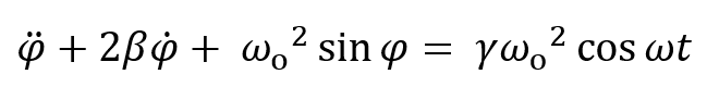
In the limit of small amplitude oscillations, this is the driven damped oscillator explored in previous applets.
But for larger oscillations, the system exhibits surprising new phenomena: period doubling and chaos, as discussed, for example in Taylor’s Classical Mechanics.
With this applet you can explore a whole range of novel behaviors: for a small sinusoidal driving force, the response is at the same frequency as the driver,
but at a certain strength, the response period doubles, and the doubling repeats at diminished intervals, and goes to infinity: that is, no period in the response, just chaos.
Yet further increases in driving strength bring back periodicities for certain strength ranges.
But why spend time examining the complex behavior of this simple-looking system?
Because, it turns out, the behavior exhibited here occurs in many, many systems, some far more complicated. The period doubling and onset of chaos have surprising universality.
Walk-Through
First, we have set the damping force and driving frequency equal to those in Taylor’s book, to verify that the applet can reproduce the computer-generated graphs he shows,
which it does. But you can set the damping force over a wide range, and explore the differences.
The variable gamma is a measure of the relative importance of the driving force compared to the gravitational torque. For gamma less than one or so, gravity dominates.
The applet is initially set for gamma = 0.9. Run the applet and note it’s fairly close to sinusoidal, even though the pendulum is swinging above the horizontal.
Note the up and down amplitudes agree to five figures after six cycles with dt = 0.0005.
Now: gamma = 1, looks similar, but takes about 100 cycles for up and down amplitudes to agree to 5 figures. Gamma = 1.05: wild initial swing, then after four cycles or so,
settles down, but around 4 pi (it did two circles). (Type these numbers in: 1.051 will give different transient behavior.) Gamma = 1.06: takes 8 or so cycles to settle. 1.07: once it’s settled, track the heights of successive peaks (or dips) as
recorded in the amplitude, middle turquoise figure in bottom box (it's the most recent extremum--it will take about 50 cycles for the numbers to recur to 4 figure accuracy. Use the play speed slider to get there fast, then slow down to see what's happened). They alternate in height! You can see this visually by moving the horizontal red line (slider just under the graph). The period has doubled. Try gamma = 1.073, compare with fig 12.5 in Taylor’s book.
These initial swings are very sensitive to gamma: try varying it by 0.001.
Or, better, check out the next applet, which will plot the two curves simultaneously.
Try gamma =1.077 to find a period three final oscillating state. Now change the initial angle to -90 degrees: a quite different result!
Evidently there are (at least) two different final oscillating states possible, depending on initial conditions. Such final states are called “attractors”.
Note the resemblance of the three cycle to the initial wanderings at other gamma values. You can explore different initial angles to see what happens.
Use the amplitude readout to find further period doubling (keeping the initial angle at -90 degrees) at gamma = 1.081 there is period 4, at 1.0826 period 8, and at 1.0829 there is no periodicity: this is chaos.
Important! Near bifurcations, there are long-lived transients. Use the speed slider to speed things up: you can go to speed 50, run for hundreds or even thousands of cycles in a short time, then pause, set speed to 1 or 2, play, and read out the amplitude (the most recent extremum), to look for periodicity. The high speed doesn't affect accuracy, just prints a lot less dots. In fact, by staring at the pattern generated at speed, it's often easy to see the changes in periodicity.
Next, try different values of damping, initial angle, gamma, etc.
Here's the relevant lecture, which includes more details.
Previous applet: Driven Damped Anharmonic Oscillator.
Next applet: Driven Damped Pendulum II: plotting two curves initially close.
Program by: Carter Hedinger