22. Driven Damped Anharmonic Oscillators
Michael Fowler
Introduction
Landau’ next sections (Chapter 6, sections 28,29) address nonlinear one-dimensional systems. In particular, he focusses on driven damped oscillators with nonlinear, but small, added potential terms. Using ingenious semiquantitative techniques, he predicts some unexpected results: for example, a discontinuity in the oscillation amplitude on slowly varying the driving frequency at constant driving force (and constant damping). He also finds resonances when the driving frequency is a fraction, for example a third, of the oscillator’s natural frequency.
Fortunately, this system is easy to analyze numerically, and we have an applet to do just that. The parameters are set by sliders, and one can immediately find the large discontinuity in amplitude (factor of two or so) as the frequency is slightly changed. At the end of this lecture, we show simple plots of amplitude response to a constant driving force as the frequency is varied. These were found using the applet, the reader can easily check them, and venture into parts of the parameter space. The applet provides a measure of Landau’s (semiquantitative) accuracy, of course surprisingly good (of order 20% error or less) given the nature of the problem.
It should be added that this is one area where, thanks to computers, major advances have been made since Landau wrote the book, in particular the discovery for some systems of period doubling and chaos as the driving force is increased. We’ve added a lecture (22a) on a particular system, the driven damped pendulum, a natural extension of Landau’s oscillator. This illustrates some of the novel features. We will follow part of chapter 12 of Taylor’s excellent text, Classical Mechanics. Taylor provides many computer-generated graphs of the pendulum’s response as parameters are varied. We provide applets that can generate these graphs. The reader can easily use these applets to explore other parameter inputs.
In this lecture, to gain a bit of intuition about these nonlinear potentials, we’ll begin (following Landau) with no driving and no damping: just a particle oscillating in a potential that’s simple harmonic plus small and (positive) terms. The basic questions are, how do these terms change the frequency of oscillation, and how does that frequency depend on the amplitude of oscillation? The answers will guide us in understanding how a particle in such a potential will respond to a harmonic driving term, plus damping.
Next, we briefly review the driven damped linear oscillator (covered in detail in lecture 18, this is really just a reminder of the notation). Then we add small cubic and quartic terms. We present Landau’s argument that--above a certain driving force--gradually increasing the driving frequency leads at a critical value to a discontinuous drop in the amplitude of the response, then use an applet to confirm and quantify his result.
Frequency of Oscillation of a Particle is a Slightly Anharmonic Potential
See the applet illustrating this section.
Landau (para 28) considers a simple harmonic oscillator with added small potential energy terms . In leading orders, these terms contribute separately, and differently, so it’s easier to treat them one at a time. We’ll first consider the quartic term, an equation of motion
(We'll always take positive.)
Writing a perturbation theory expansion (following Landau):
(Standard practice in most books would be to write with the superscript indicating the order of the perturbation--we're following Landau's notation, hopefully reducing confusion…)
We take as the leading term
with the exact value of , . Of course, we don’t know the value of yetthis is what we’re trying to find!
And, as Landau points out, you can’t just write because that implies motion increasing in time, and our system is a particle oscillating in a fixed potential, with no energy supply. Furthermore, even if we did somehow have the value of exactly right, this expression would not be a full solution to the equation: the motion is certainly periodic with period , but the complete description of the motion is a Fourier series including frequencies an integer, since the potential is no longer simple harmonic.
Anyway, putting this correct frequency into the equation of motion gives a nonzero left-hand side, so we rearrange. We subtract from both sides to get:
Now putting the leading term into the left-hand side does give zero: if the equation had zero on the right hand side, this would just be a free (undamped) oscillator with natural frequency not This doesn’t look very promising, but keep reading.
The equation for the first-order correction is:
Notice that the second term on the right-hand side includes . This equation now represents a driving force on an undamped oscillator exactly at its resonant frequency, so would cause the amplitude to increase linearly, obviously an unphysical result, since we’re just modeling a particle sliding back and forth in a potential, with no energy being supplied from outside!
The key is that there is also a resonant driver in that first term
Clearly these two driving terms have to cancel, and this requirement nails : here’s how:
so the resonant driving terms cancel provided
Remembering , this gives (to this order)
(Strictly, in the denominator, but that’s a higher order correction.)
Note that the frequency increases with amplitude: the potential gives an increasingly stronger restoring force with amplitude than the harmonic well. You can check this with the applet.
Now let’s consider the equation for a small cubic perturbation,
This represents an added potential which is an odd function, so to leading order it won’t change the period, speeding up one half of the oscillation and slowing the other half the same amount in leading order. The first correction to the position as a function of time is the solution of
The solution is
Physically, adding this to the leading term, the particle is spending more of its time in the softer half of the potential, giving an amplitude-dependent correction to its average position.
To get the correction to the frequency, we need to go to the next order, Dropping terms of higher order, the equation of motion for the next correction is
and with following Landau,
Again, there cannot be a nonzero term driving the system at resonance, so the quantity in the square brackets must be zero, this gives us
The total correction to frequency to leading order for the additional small potentials is therefore (they add independently to this order)
(the here being a convenient notation Landau employs later).
How Good Are These Approximations?
We have an applet that solves this equation numerically, so it is straightforward to check.
Beginning with the quartic perturbation potential Landau finds a frequency correction Taking a rather large perturbation we find from the applet that whereas Landau’s perturbation theory predicts However, if we correct Landau’s denominator (as mentioned above, he pointed out it should be but said that was second-order) the error is very small.
Taking the formula gives so less than two percent error, and for amplitude 0.2, the effort is less than 0.1%.
Explore with the applet here.
Resonance in a Damped Driven Linear Oscillator: A Brief Review
This is just to remind you of what we covered in lecture 18, before we add anharmonic terms in the next section.
The linear damped driven oscillator has equation of motion:
(Following Landau’s notation herenote it means the actual frictional drag force is )
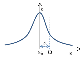
Looking near resonance for steady state solutions at the driving frequency, with amplitude , phase lag , that is, , we find
For a near-resonant driving frequency
and assuming the damping to be sufficiently small that we can drop the term along with , the leading order terms give
so the response, the dependence of amplitude on driving frequency is to this accuracy
(Note also that the resonant frequency is itself lowered by the damping, another second-order effect we’ll ignore.)
The rate of absorption of energy equals the frictional loss. The friction force on the mass moving at is doing work at an average rate:
The half width of the resonance curve as a function of is given by the damping. The total area under the curve is independent of damping.
For future use, we’ll write the above equation for the amplitude in terms of deviation from the resonant frequency
Damped Driven Nonlinear Oscillator: Qualitative Discussion
We now add to the damped driven linear oscillator a positive quartic potential term, giving equation of motion
As mentioned above, for a particle oscillating in this potential the frequency increases with amplitude: the bigger swings encounter a potential becoming stronger and stronger than the simple harmonic oscillator.
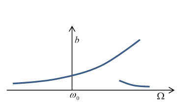
So if we drive the oscillator from rest at the frequency that resonates with its small amplitude oscillations (where the potential term has negligible effect), as the amplitude builds up, the oscillator frequency increases, and the driving force falls out of sync.
The way to keep the amplitude increasing is evidently to gradually increase the frequency of the driving force to match the natural frequency at the increased amplitude. (Side note: this is the principle of the synchrocyclotronexcept, in that case the frequency is lowered as the energy increases, because the particles go to bigger and bigger orbits as their mases increase relativistically.) This way a small external driving force (enough to overcome frictional damping) can maintain a large amplitude oscillation at a frequency well above the frequency of small oscillations.
But what if we apply this high frequency to a system initially at rest, rather than gradually ramping up in sync with the oscillations? Then for a small driving force, we can treat the system as a damped simple harmonic oscillator, and this off-resonance force will drive relatively small amplitude oscillations.
The bottom line is that for the same external driving force, with frequency in some range above , there can be two possible steady state oscillation amplitudes, depending on the history of the system.
Nonlinear Case: Landau’s Analysis
The equation of motion is:
We established earlier that the nonlinear quartic term brings in a correction to the oscillator’s frequency that depends on the amplitude :
in Landau’s notation,
The equation for the amplitude in the linear case (from the previous section) was, with
For the nonlinear case, the maximum amplitude will clearly be at the true (amplitude dependent!) resonance frequency so with as before, we now have a cubic equation for :
.
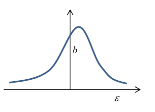
Note that for small driving force is small ( ) but the center of the peak has shifted slightly upwards, to that is, at a driving frequency The cubic equation for has only this one real solution.
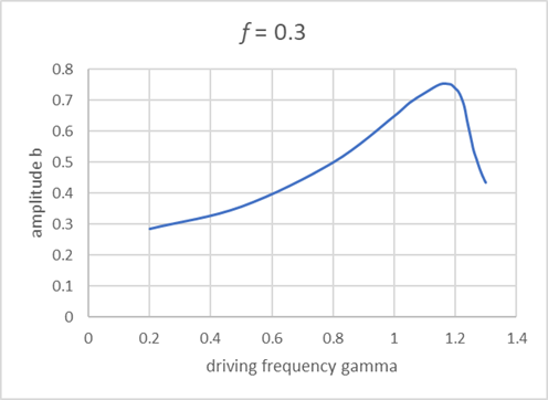
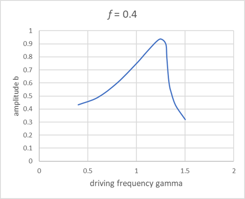
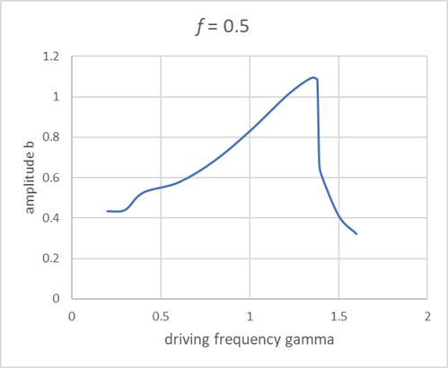
However, as the driving force is increased, the coefficients of the cubic equation change and at a critical force two more real roots appear.
The curve for driving force above looks like:
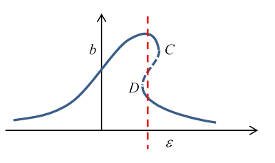
So what’s going on here? For a range of frequencies, including the vertical dashed red line in the figure, there appear to be three possible amplitudes of steady oscillation at one frequency. However, it turns out that the middle one is unstable, so will exponentially deviate, going to one of the other two, both of which are stable.
If the oscillator is being driven at , and the driving frequency is gradually increased, the amplitude will follow the upper curve to the point , then drop discontinuously to the lower curve. Further frequency increase (with the same strength driving force, of course) will give diminishing amplitude of oscillationjust as happens for the ordinary simple harmonic oscillator on going away from the resonant frequency.
If the frequency is now gradually lowered, the amplitude gradually will increase to point , where it will jump discontinuously to the upper curve. The overall response to driving frequency is sometimes called hysteresis, by analogy with the response of a magnetic material to a varying imposed external field.
To put in some numbers, the maximum amplitude for any of these curves is when that is, at or
the same result as for small oscillations.
To find the critical value of the driving force for which the multiple solutions appear, in the graph above that’s when coincide. That is, has coincident roots.
Differentiating the equation for amplitude as a function of frequency (and of course this is at constant driving force )
coincide when the discriminant in the denominator quadratic is zero, that is, at where
Putting these values into the equation for as a function of driving force the critical driving force is
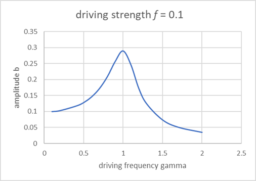
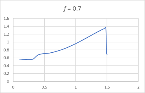
Numerical Applet Results
The results above are all from Landau’s book, and are semiquantitative. They can easily be checked using our online applet, which is accurate to one percent or better. The curves below are plotted from applet results, and certainly exhibit the behavior predicted by Landau.
These plots are for
For these values, Landau's is approximately 0.3. Ours looks a bit more. Note for we show close to graph peak.
Frequency Multiples
The above analysis is for frequencies not very far from . But nonlinear terms can cause resonance to occur at frequencies which are rational multiples of . Landau shows that a small in the potential (so an additional force in the equation of motion) can generate a resonance near . We’ve only considered a quartic addition to the potential, , a force , we can show that gives a resonance near and presumably this is the small bump near the beginning of the curves above for large driving strength.
We have
We’ll write
Let’s define by
So . Then
Then, for , the second term, , will have a resonant response, although it is proportional to the (small) amplitude cubed.
Similar arguments work for other fractional frequencies.