previous  index  next 

4. Math Bootcamp

    Michael Fowler, UVa

Introduction

 Here we’ll first review basic vector calculus: grad, div, curl, Gauss’ theorem, Stokes’ theorem and their variants.   This is essential material for graduate E&M!  Another crucial tool for understanding these fields is the Fourier transform, which also introduces in a natural way Dirac’s indispensable delta function, discussed at the end of the lecture.

Vectors: Cartesian Coordinates, Kronecker Delta

In E&M (in contrast to, say, QM) our vectors are not in an abstract space, they’re in three dimensions.

The essential properties of a linear vector space are that addition and multiplication by a scalar (a number) are defined and give another vector in the space.  

Our ordinary three-dimensional space is spanned by three orthonormal basis vectors, the unit vectors along the $x,y,z$ axes, often written $\widehat{\overrightarrow{x}},\widehat{\overrightarrow{y}},\widehat{\overrightarrow{z}}$.  

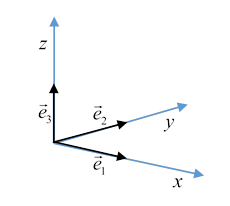
For notational efficiency, it is often convenient to write these unit vectors ${\overrightarrow{e}}_1,{\overrightarrow{e}}_2,{\overrightarrow{e}}_3,$ and their mutual orthogonality

${\overrightarrow{e}}_i\cdot {\overrightarrow{e}}_j={\delta }_{ij},$ 

this ${\delta }_{ij}$ is called the Kronecker delta: it’s equal to 1 if $i=j$, zero if $i\ne j$. 

Dummy Suffixes

Any 3D vector is a sum over components$—$the basis vectors ${\overrightarrow{e}}_i$ are said to “span the space”:

$\overrightarrow{a}=a_x\widehat{\overrightarrow{x}}+a_y\widehat{\overrightarrow{y}}+a_z\widehat{\overrightarrow{z}}\equiv a_1{\overrightarrow{e}}_1+a_2{\overrightarrow{e}}_2+a_3{\overrightarrow{e}}_3=a_i{\overrightarrow{e}}_i,$ 

where we’ve introduced Einstein’s dummy suffix notation in that last step:

If a suffix appears twice in an expression, the sum over 1,2,3 is understood. 

If the same suffix appears more than twice, you made a mistake$—$the expression is meaningless.  

The position vector

$\overrightarrow{r}=\left(x,y,z\right)=\left(x_1,x_2,x_3\right)$ 

 becomes

$\overrightarrow{r}=x_i{\overrightarrow{e}}_i.$ 

(It is also often written $r_i{\overrightarrow{e}}_i.$ )

The magnitude of the vector is written

$\left|\overrightarrow{a}\right|=\sqrt{a_1^2+a_2^2+a_3^2}=\sqrt{a_i{a}_i}.$ 

 (You may be aware that in general relativity, this would be written $\sqrt{a_i{a}^i},$ and summation is only allowed between up and down indices.  This refinement is unnecessary in E&M in ordinary space, that is, not gravitationally warped space).

Rotating a Displacement Vector, Orthogonal Matrices

Consider the incremental displacement vector

$\Delta \text{}\overrightarrow{x}=\left(\Delta x_1,\Delta x_2,\Delta x_3\right).$ 

We know how this transforms under a rotation: for example, a rotation of the displacement vector about the $z$ axis gives new components in the fixed frame of reference:

$\left(\begin{array}{c}\Delta {x^{\prime }}_1\\ \Delta {x^{\prime }}_2\\ \Delta {x^{\prime }}_3\end{array}\right)=\left(\begin{array}{ccc}\cos \theta & -\sin \theta & 0\\ \sin \theta & \cos \theta & 0\\ 0& 0& 1\end{array}\right)\left(\begin{array}{c}\Delta x_1\\ \Delta x_2\\ \Delta x_3\end{array}\right)$ .

(One way to see this is to write $\Delta \overrightarrow{x}$ as a sum of three vectors, each along an axis, then rotate them separately, and write down their new components, then add.)

However, confusingly, a more common transformation is to find the new components of a fixed vector in a new frame of reference, which is, say, the old frame of reference rotated by $\theta$ about the $z$ axis. This is of course

$\left(\begin{array}{c}\Delta {x^{\prime }}_1\\ \Delta {x^{\prime }}_2\\ \Delta {x^{\prime }}_3\end{array}\right)=\left(\begin{array}{ccc}\cos \theta & \sin \theta & 0\\ -\sin \theta & \cos \theta & 0\\ 0& 0& 1\end{array}\right)\left(\begin{array}{c}\Delta x_1\\ \Delta x_2\\ \Delta x_3\end{array}\right).$ 

(It's worth mentally checking for a small angle to be sure you've got this sign right.)

This is an orthogonal matrix: it transforms orthogonal vectors into orthogonal vectors, its transpose is its inverse, obvious from the form above.

Since a general rotation can be written as a succession of rotations around axes,  $A^{-1}=A^T$ for any rotation.

Exercise:  Prove that if $A^{-1}=A^T,B^{-1}=B^T$ then ${\left(AB\right)}^{-1}={\left(AB\right)}^T.$

We’ll write the general rotation matrix as

$\Delta {x^{\prime }}_i=R_{ij}\Delta x_j.$ 

Regarding the displacements as infinitesimals, we see that the transformation can be written

$d{x^{\prime }}_i=\frac{\partial {x^{\prime }}_i}{\partial x_j}d{x}_j$ 

and of course from the chain rule,

$\frac{\partial {x^{\prime }}_i}{\partial x_j}\frac{\partial x_j}{\partial {x^{\prime }}_k}=\frac{\partial {x^{\prime }}_i}{\partial {x^{\prime }}_k}={\delta }_{ik}.$ 

From this, we can deduce that for a rotational change of basis, the differential operator transforms as

$\frac{\partial }{\partial {x^{\prime }}_i}=\frac{\partial x_j}{\partial {x^{\prime }}_i}\frac{\partial }{\partial x_j}.$ 

We’ll return to this soon.

Definition of a Vector

It’s not just those three numbers$—$a vector isn’t given just by specifying its components in one frame of reference, there has to be a prescription for finding its components in any frame of reference.

So we define a vector $\overrightarrow{a}$ having components $\left(a_1,a_2,a_3\right)$ in one frame and by requiring that the components in a new frame are given by exactly the same linear transformation that gives the components of a displacement vector $\Delta \overrightarrow{x}$ in the new frame in terms of the components $\left(\Delta x_1,\Delta x_2,\Delta x_3\right)$ in the original frame, that is, as discussed above,  $\Delta {x^{\prime }}_i=R_{ij}\Delta x_j.$  

Hence by definition, under rotation the components of a vector $\overrightarrow{a}$ transform by

${a^{\prime }}_i=R_{ij}{a}_j.$ 

Definition of a Tensor

For future reference, we'll mention here what are called Cartesian tensors. The vector has the single suffix $i,$ as in $a_i,$ a tensor has two or more suffixes, hence 9, 27, etc. components in three dimensions.

Each component transforms exactly as does the single$–$suffix vector, meaning that under rotation,  when for a vector ${a^{\prime }}_i=R_{ij}{a}_j,$ for a second-rank (two suffixes) tensor

${T^{\prime }}_{ij}=R_{ik}{R}_{jl}{T}_{kl}.$ 

Each suffix transforms by the vector rule.  We’ll soon come across important tensors.

Finally, it’s worth asking: what are the eigenvectors of a rotation matrix?  Let’s look at the one above, for rotation about the $z$ axis. Obviously, the only vector unaffected is one in the $z$ direction!  But it’s a 3X3 matrix, so two other vectors must be just multiplied by a number$—$the eigenvalue$—$and stay pointing in the same direction.  To see how that can be, we have to solve the eigenvalue equation

$\left(\begin{array}{ccc}\cos \theta & \sin \theta & 0\\ -\sin \theta & \cos \theta & 0\\ 0& 0& 1\end{array}\right)\left(\begin{array}{c}{x}_1\\ x_2\\ x_3\end{array}\right)=\lambda \left(\begin{array}{c}{x}_1\\ x_2\\ x_3\end{array}\right)$ 

from which $\left(1-\lambda \right)\left({\lambda }^2-2\lambda \cos \theta +1\right)=0,\lambda =1,e^{i\theta },e^{-i\theta }.$ 

The $\lambda =1$ result has eigenvector $\left(0,0,1\right)$, just the axis of rotation, the others are $\left(1,i,0\right),\left(1,-i,0\right).$ That's why we couldn't see them$—$they're in complex three-space. 

Exercise: check explicitly that these are indeed eigenvectors.

In fact, these eigenvectors correspond to the states of a spin one particle in quantum mechanics, and they are also relevant in describing circularly polarized light, as we shall see.

Dot Product

The scalar or dot product of two vectors is

$\overrightarrow{a}\cdot \overrightarrow{b}=a_i{b}_i,$ 

using the dummy suffix notation. 

Note that the property $R^{-1}=R^T$ guarantees that inner products, including vector length $\left|\overrightarrow{a}\right|=\sqrt{a_i{a}_i},$  will be preserved under transformation to another orthogonal base.

Check this:  write ${a^{\prime }}_i=R_{ij}{a}_j,{b^{\prime }}_i=R_{ij}{b}_j$ show ${a^{\prime }}_i{b^{\prime }}_i=a_i{b}_i.$

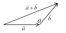
Evaluating ${\left(\overrightarrow{a}+\overrightarrow{b}\right)}^2$ makes clear that the dot product $\overrightarrow{a}\cdot \overrightarrow{b}=ab\cos \theta ,$ where $\theta$ is the angle between the vectors, also it’s evidently the component of one vector in the direction of the other, multiplied by that vector’s magnitude.

 

Cross Product, Levi-Civita Symbol, Triple Product

The vector or cross product of two vectors

$\overrightarrow{a}\times \overrightarrow{b}=\left(a_2{b}_3-a_3{b}_2,a_3{b}_1-a_1{b}_3,a_1{b}_2-b_1{a}_2\right).$ 

This cross product is written more succinctly using the Levi-Civita symbol, ${\epsilon }_{ijk}$. 

Here the suffixes $i,j,k$ go over the values 1,2,3; and ${\epsilon }_{123}={\epsilon }_{231}={\epsilon }_{312}=1,$ the counter clockwise ${\epsilon }_{132}={\epsilon }_{321}={\epsilon }_{213}=-1$ and if any two suffixes are equal, $\epsilon =0$.

Thus

${\left(\overrightarrow{a}\times \overrightarrow{b}\right)}_i={\epsilon }_{ijk}{a}_j{b}_k,$ 

( $j,k$ being summed-over dummy suffixes.)

 This has a simple geometric interpretation: taking the two vectors to have a common end (say, the origin) see them as two adjacent sides of a parallelogram.  The vector $\overrightarrow{a}\times \overrightarrow{b}$ has magnitude equal to the area of this parallelogram, and direction perpendicular to the plane. 

The sign has to be fixed by convention: it's defined to be the direction of progress of a right-handed corkscrew, the handle being rotated from $\overrightarrow{a}$ to $\overrightarrow{b}.$ 

Note that $\overrightarrow{a}\times \overrightarrow{b}=-\overrightarrow{b}\times \overrightarrow{a}.$ 

The triple product $\left(\overrightarrow{a}\times \overrightarrow{b}\right)\cdot \overrightarrow{c}$ is a scalar with magnitude equal to the volume of the parallelepiped having the three vectors as edges with their (non-arrowhead) ends at the same corner. Think of it as base area times height: the dot product of $\overrightarrow{c}$ with $\overrightarrow{a}\times \overrightarrow{b}$ equals the base area $\left|\overrightarrow{a}\times \overrightarrow{b}\right|$ multiplied by the component of $\overrightarrow{c}$ perpendicular to the base area plane$—$and that’s the height of the parallelepiped.

An Important Identity

A triple product that often comes up in E&M is

$\overrightarrow{a}\times \left(\overrightarrow{b}\times \overrightarrow{c}\right)=\overrightarrow{b}\left(\overrightarrow{a}\cdot \overrightarrow{c}\right)-\overrightarrow{c}\left(\overrightarrow{a}\cdot \overrightarrow{b}\right).$ 

This is easily proved using the important identity

${\epsilon }_{ijk}{\epsilon }_{ilm}={\delta }_{jl}{\delta }_{km}-{\delta }_{jm}{\delta }_{kl}.$ 

This identity can be established by listing possible values$—$there aren't that many, remember the $\epsilon$ 's are zero if two suffixes are the same.  Do it!

It's also worth thinking about the vector identity geometrically:  $\overrightarrow{a}\times \left(\overrightarrow{b}\times \overrightarrow{c}\right)$ must be in the $\overrightarrow{b},\overrightarrow{c}$ plane, since it's perpendicular to $\overrightarrow{b}\times \overrightarrow{c},$ so it's some linear combination of $\overrightarrow{b},\overrightarrow{c},$ and it must be perpendicular to $\overrightarrow{a}.$ 

What’s a Vector Field?

A vector field is generalization of an ordinary function $f\left(\overrightarrow{r}\right)$.

An ordinary function assigns a number to each point in the space where it’s defined, for example a map of temperature over an area (or even a volume). 

A vector field gives a vector for each point in some space, such as $\overrightarrow{E}\left(\overrightarrow{r}\right)=\frac{1}{4\pi {\epsilon }_0}\frac{q\widehat{\overrightarrow{r}}}{r^2},r\ne 0$. 

Exercise:  sketch roughly the magnetic field for a small bar magnet.  That’s a vector field: strictly, there’s an arrow at each point in space.

What we’ve called an ordinary function is often called a scalar function or scalar field, to contrast it with a vector field.  The electrostatic potential in some volume is a scalar field.

The Gradient Operator

Definition

The gradient operator, called grad, is

$\overrightarrow{\nabla }=\widehat{\overrightarrow{x}}\frac{\partial }{\partial x}+\widehat{\overrightarrow{y}}\frac{\partial }{\partial y}+\widehat{\overrightarrow{z}}\frac{\partial }{\partial z}={\overrightarrow{e}}_i\frac{\partial }{\partial x_i}.$

To picture the gradient operator, we’ll look at a two-dimensional example: a contour map of a stretch of territory with mountains, etc. 

 

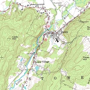
The many lines on the map connecting points at the same height are called contours.   Essentially, the map shows height as a function of latitude and longitude, we’ll use $\left(x,y\right)$ coordinates from some local origin, so the height is a scalar function $h\left(x,y\right)$. 

Then $\overrightarrow{\nabla }h\left(x,y\right)$ is a vector field, giving, in fact, the local gradient in the usual geographic sense, that is, rate of change of height with respect to change in horizontal position.

If you take a step on this terrain $\Delta \overrightarrow{r}=\left(\Delta x,\Delta \text{}y\right)$ your change in altitude is $\overrightarrow{\nabla }h\cdot \Delta \overrightarrow{r}.$ 

Exercise:  Check from the transformation laws given above that $\Delta \overrightarrow{r}\cdot \overrightarrow{\nabla }f$ is invariant under rotations, and interpret your result.  Now prove that taking a walk and coming back, ${\displaystyle \underset{\text{closed path}}{\oint }\overrightarrow{\nabla }h\cdot d\overrightarrow{r}=0}$.

Evidently, $\overrightarrow{\nabla }h$ is a vector field in the two-dimensional space, and in fact it’s just the component of the gravitational field for motion confined to the surface (the other is cancelled by the normal force holding you to the surface), that is, $mg\overrightarrow{\nabla }h\cdot d\overrightarrow{r}$ is the work you do against gravity when you take the small step with horizontal components $d\overrightarrow{r}$, this expression is the increase in your gravitational potential energy.

Equipotentials and the Gradient Operator

The lines of constant height on a geographical map, the contour lines mentioned above, are clearly gravitational equipotentials, it takes no work against gravity to walk around at constant height, your potential energy doesn’t change, so, as we've found, for a step $d\overrightarrow{r}$ along such a line we must have $\overrightarrow{\nabla }h\cdot d\overrightarrow{r}=0$.

That is to say, the vector field $\overrightarrow{\nabla }h$ is perpendicular to the equipotential lines everywhere, it’s pointing along the line of maximum slope (often called steepest descent).  Analogously, the direction of the electric field at a point in an electrostatic problem is always perpendicular to the equipotential surface (this is three dimensions) through that point.

Exercise: (We'll be doing this in more detail later, this is to check you get the idea.)  Sketch equipotentials and field lines for a system of two equal magnitude charges: same charge, opposite charge.  In particular, sketch the lines near a saddle point: the midpoint between two like charges.

The Divergence Operator: Definitions, Gauss’ Theorem, Visualization

Definition

The divergence (called div) is formally defined as the differential operator acting on a vector field:

$\overrightarrow{\nabla }\cdot \overrightarrow{V}=\frac{\partial V_x}{\partial x}+\frac{\partial V_y}{\partial y}+\frac{\partial V_z}{\partial z}=\frac{\partial V_i}{\partial x_i}.$

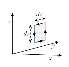
There’s another way to define divergence: take a tiny cubical box, sides $dx,dy,dz$ around some point $\left(x,y,z\right)$ then

$\overrightarrow{\nabla }\cdot \overrightarrow{V}\left(x,y,z\right)=\underset{dx,dy,dz\to 0}{\lim }\frac{{\displaystyle \underset{\text{surface of cube}}{\int }\overrightarrow{V}\cdot d\overrightarrow{S}}}{dxdydz}$

Here $d\overrightarrow{S}$ is a vector representing an increment of surface area$—$its magnitude is the area, its direction is perpendicular to the surface, but we have to specify which way, for a closed surface the convention is almost always outwards.

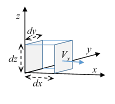
Let’s check that the two definitions are equivalent: consider first the contribution to the surface integral from the two faces perpendicular to the $x$ axis, they have areas of magnitude $dydz$.  In the limit of a small box, we can assume the variation of $\overrightarrow{V}$ on these faces in the $y,z$ directions can be neglected, but the variation between the two faces because they are separated by $dx$ is the only contribution to the integral, since the $d\overrightarrow{S}$ for the two faces are in opposite directions, $\pm \widehat{\overrightarrow{x}}$.

Hence the net contribution to the integral over the cube surface from those faces is $\frac{\partial V_x}{\partial x}dx$ multiplied by the area $dydz$, and the product of infinitesimals $dxdydz$ cancels with the denominator (in the expression for $\overrightarrow{\nabla }\cdot \overrightarrow{V}$ above) leaving just $\partial V_x/\partial x$. The two other pairs of faces make corresponding contributions, establishing the equivalence of the two definitions.

Gauss’ Theorem

Gauss’ Theorem, a. k. a. the Divergence Theorem, is:

${\displaystyle \underset{V}{\int }{d}^{3}r\overrightarrow{\nabla }\cdot \overrightarrow{F}}={\displaystyle \underset{S}{\int }d\overrightarrow{S}\cdot \overrightarrow{F}}.$

This easily follows from the “small box” definition of the divergence: divide the whole volume into tiny boxes, so the volume integral is a surface integral over these myriads of surfaces.  But the integrals over the internal surfaces all cancel, leaving just that over the bounding surface.

Visualizing Divergence:  Velocity Field for an Incompressible Fluid

To picture what the divergence of a vector field can look like, it’s helpful to visualize the flow of an incompressible fluid, with the velocity vector field $\overrightarrow{v}\left(\overrightarrow{r}\right).$  Let’s assume at the moment that it’s a steady flow, not varying in time. Obviously, if the fluid is incompressible, it can’t be piling up anywhere, and we’ll assume there are no bubbles, it fills all the space we’re considering.  (We’re taking the density of the fluid to be $\rho =1$, so the velocity field is the same as mass flow$—$remember the fluid is incompressible.) 

Then, from the small cube picture, as much is flowing into any space as is flowing out, $\overrightarrow{\nabla }\cdot \overrightarrow{v}=0$ everywhere.  How do we change that?  By having a source of fluid.

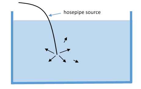
Consider a large body of water, like a deep large pool, and slip a thin hosepipe in, so the end is deep in the water somewhere. Now pump in water at a steady rate. Once things have settled down, if you imagine any surface within the water that encloses the source, ${\displaystyle \underset{}{\int }\overrightarrow{v}\cdot d\overrightarrow{S}}$ over that surface must equal the rate of supply of water, call it $q$.

If the water is at rest apart from the motion caused by this supply, $\overrightarrow{v}$ will point outwards symmetrically from the source, and the surface integral, now taken over a sphere, will tell us that $\overrightarrow{v}=q\widehat{\overrightarrow{r}}/4\pi r^2$.  Furthermore, $\overrightarrow{\nabla }\cdot \overrightarrow{v}$ is zero everywhere except at the source, where it’s evidently large.  (We’re assuming the walls are far away and we are ignoring them.)

This is of course the pattern of the electric field from a localized charge distribution.  We see that $\overrightarrow{\nabla }\cdot \overrightarrow{v}$ at the hose is the local rate of water supply, integrating over the finite volume of the hose nozzle gives the total supply.  Similarly, the divergence of the electric field gives the local charge density: the first of Maxwell’s equations is

$\overrightarrow{\nabla }\cdot \overrightarrow{E}=\frac{\rho }{{\epsilon }_0}.$ 

 A negative charge, in our watery analogy, is like a hosepipe with water being pumped away: imagine the flow field for two hoses not far from each other, one supplying water, the other taking it away.   This is like two opposite charges.

A truly point charge has its problems, mathematically and physically, which we’ll discuss later.  What about a uniformly charged (throughout its volume) sphere?  That has uniform nonzero divergence inside it, and it’s an easy exercise using the divergence theorem to find that the spherically symmetric electric field increases linearly from zero at the center, to the sphere’s surface, then falls off as the inverse square.  (This is the same as the gravitational field inside and outside the Earth, apart from sign, and assuming a uniform-density Earth.)

Variations of Gauss’ Theorem

Consider the abstract vector field $\overrightarrow{F}\left(\overrightarrow{r}\right)=\overrightarrow{c}p\left(\overrightarrow{r}\right)$ where $\overrightarrow{c}$ is a constant vector, and $p\left(\overrightarrow{r}\right)$ a scalar function of position. Gauss' theorem for this field is

$\overrightarrow{c}\cdot {\displaystyle \underset{S}{\int }pd\overrightarrow{S}}=\overrightarrow{c}\cdot {\displaystyle \underset{V}{\int }\overrightarrow{\nabla }p{d}^{3}r}.$

Exercise:  Think about $p\left(\overrightarrow{r}\right)$ as the local pressure in a fluid at rest under gravity.  Take some volume completely inside the fluid, and interpret the equation physically.

More variations:  writing Gauss’ theorem as

${\displaystyle \underset{V}{\int }{d}^{3}r{\partial }_i{F}_i}={\displaystyle \underset{S}{\int }da{n}_i{F}_i},$ 

where $n_i$ is the unit vector pointing outwards, we see that we can formally replace the $F_i$ by a tensor $F_{ij}$ or $F_{ijk},$ etc., to get

${\displaystyle \underset{V}{\int }{d}^{3}r{\partial }_i{F}_{ij}}={\displaystyle \underset{S}{\int }da{n}_i{F}_{ij}},$ 

because this is just the divergence theorem repeated three times, for $j=1,2,3.$ 

The Curl Operator: Definitions, Stokes’ Theorem, Visualizations

Definition

The curl is:

$\overrightarrow{\nabla }\times \overrightarrow{V}=\widehat{\overrightarrow{x}}\left(\frac{\partial V_z}{\partial y}-\frac{\partial V_y}{\partial z}\right)+\widehat{\overrightarrow{y}}\left(\frac{\partial V_x}{\partial z}-\frac{\partial V_z}{\partial x}\right)+\widehat{\overrightarrow{z}}\left(\frac{\partial V_y}{\partial x}-\frac{\partial V_x}{\partial y}\right).$

This rather cumbersome expression is more succinctly written using the Levi-Civita symbol, ${\epsilon }_{ijk}$ introduced earlier.  Recall, the suffixes $i,j,k$ go over the values 1,2,3; and ${\epsilon }_{123}={\epsilon }_{231}={\epsilon }_{312}=1,$ the counter clockwise ${\epsilon }_{132}={\epsilon }_{321}={\epsilon }_{213}=-1$ and if any two suffixes are equal, $\epsilon =0$.

So switching from $x,y,z$ to 1,2,3,

${\left(\overrightarrow{\nabla }\times \overrightarrow{V}\right)}_i={\epsilon }_{ijk}\frac{\partial }{\partial x_j}{V}_k.$ 

And, just as for the div, there’s an integral way to express this:

To find the component of the curl in a particular direction, we take a small square contour perpendicular to that direction (so its area $d\overrightarrow{S}$ is in that direction) and find the limit of a line integral of the vector field around that contour as the contour size goes to zero, then divide the result by the area of the square. 

So for the $x$ component,

${\left(\overrightarrow{\nabla }\times \overrightarrow{V}\left(x,y,z\right)\right)}_x=\underset{dy,dz\to 0}{\lim }\frac{{\displaystyle \underset{\text{perimeter of square}}{\int }\overrightarrow{V}\cdot d\overrightarrow{l}}}{dydz}$ 

The argument is closely parallel to that for the divergence, now we take opposite sides together, they nearly cancel, etc.: left as an exercise for the reader.

Stokes’ Theorem

This definition leads easily to Stokes’ Theorem relating an integral over an open surface to an integral around its boundary:

${\displaystyle \underset{S}{\int }d\overrightarrow{S}\cdot \overrightarrow{\nabla }\times \overrightarrow{F}}={\displaystyle \underset{C}{\oint }d\overrightarrow{l}\cdot \overrightarrow{F}}.$ 

Now we divide the surface into many small squares, taking the sum of the line integrals around all of them, all the interior parts cancel in pairs, leaving the integral around the perimeter, the curve $C$, the edge of the surface $S$.

The Electrostatic Field Has Zero Curl

Evidently, since ${\displaystyle \underset{C}{\oint }\overrightarrow{E}\cdot d\overrightarrow{l}}$ is the change in potential on going around a closed circuit, zero, an electrostatic field from a point charge has zero curl everywhere, and therefore so does any other electrostatic field, since experimentally it’s found that electric fields just add linearly. 

This is really equivalent to saying that any electrostatic field is the gradient of a single-valued potential,

$\overrightarrow{E}\left(\overrightarrow{r}\right)=-\overrightarrow{\nabla }\phi \left(\overrightarrow{r}\right),$ 

it’s easy to see that $\overrightarrow{\nabla }\times \overrightarrow{E}=-\overrightarrow{\nabla }\times \overrightarrow{\nabla }\phi =-{\epsilon }_{ijk}\frac{{\partial }^2\phi }{\partial x_j\partial x_k}=0$ from the antisymmetry ${\epsilon }_{ijk}=-{\epsilon }_{ikj}$.

(Nitpicking note: We’ll soon see that zero curl only necessarily means the field is a gradient if the space is simply connected.)

Visualizing Curly Fields: A Whirlpool in Incompressible Fluid and its Magnetic Analog

From this picture of the curl as the limit of an integral around a small contour, divided by the area enclosed by the contour, can that be visualized as the flow field of some incompressible fluid?

(The motivation here is visualizing the magnetostatic (time-independent) field, for which Maxwell’s second equation, $\overrightarrow{\nabla }\cdot \overrightarrow{B}=0,$ assures us a sourceless incompressible fluid scenario will be valid)  Furthermore, for static fields we have $\overrightarrow{\nabla }\times \overrightarrow{B}={\mu }_0\overrightarrow{j}$, $\overrightarrow{j}$ being the current density.)

Consider the velocity field from a whirlpool. We’ll just keep to two dimensions for simplicity, looking at the surface, say of an emptying bathtub over the drain, or a hurricane viewed from a satellite. Clearly now ${\displaystyle \underset{\text{circle}}{\oint }\overrightarrow{v}\cdot d\overrightarrow{l}}\ne 0$ for a circle centered at the origin, there's a whirlpool.  In fact, for an incompressible inviscid fluid in steady rotational motion of this type, Kelvin proved that the integral

${\displaystyle \underset{\text{circle}}{\oint }\overrightarrow{v}\cdot d\overrightarrow{l}}=K,$ 

 a path-independent constant for any contour including the origin. $K$ is called the circulation.  It follows that the integral is zero if the closed contour does not include the origin, and that means $\overrightarrow{\nabla }\times \overrightarrow{v}=0$ for this flow except at the origin, where it is a two-dimensional delta function of strength $K.$  

In fact, this velocity field is the same as the magnetic field from a steady current in a long straight wire: that goes down as $1/r$ with distance from the wire.

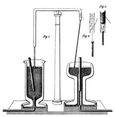
Obviously, this field cannot be represented as the gradient of a single-valued potential: if we had a magnetic monopole, and allow it to move on a circular track around the wire, it would circle around with more and more energy!  Actually that scenario is essentially equivalent to one of Faraday’s first electric motors: (the one on the right in the illustration) he had a long vertical bar magnet, the north pole above the surface of a pool of mercury, the south pole far below, and a current-carrying wire suspended from a point vertically above the north pole, its end in the mercury. The wire rotated in the mercury.

Exercise:  Where is the energy to keep the wire rotating coming from?  And, what’s going on on the left side of the illustration?

Evidently, although $\overrightarrow{\nabla }\times \overrightarrow{B}=0$ everywhere outside the wire, this doesn’t guarantee that $\overrightarrow{B}=\overrightarrow{\nabla }\psi ,$ for some scalar potential, obviously it isn’t. 

Contrasting Different Curly Vector Fields: The Whirlpool and The Rotating Solid Body

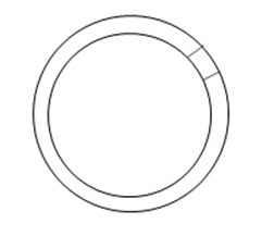
Let’s think a bit more about the curl of the velocity field of a whirlpool: all the velocity lines move in circles, it looks a bit curly. But to check, take a small contour between two adjacent circles, with radial ends, which won’t contribute to the integral. Around the curved sides, the speed goes as $1/r$, but the length of contour goes as $r$, so the two contributions to the contour integral from the curved sides cancel, meaning this flow field has zero curl (except at the central point).

Now contrast this with the velocity field of a rotating solid body: taking the same little contour, the contributions from the curved sides, using $v=\omega r$,  will be

$\omega {\left(r+dr\right)}^{2}d\theta -\omega r^{2}d\theta$ 

from which $\overrightarrow{\nabla }\times \overrightarrow{v}=2\omega \widehat{\overrightarrow{z}}$, where $\widehat{\overrightarrow{z}}$ is a unit vector along the axis of rotation: the velocity curl has uniform magnitude throughout the rotating body.

In fact, this uniform curl describes the magnetic field inside a thick wire carrying a current, provided the current density is uniform over the whole cross-section.

A useful way to see the difference between these two circulating fields (whirlpool and rotating body) is to visualize the motion of a small piece of paper floating on the fluid surface. The rotation of the piece of paper measures the local curl of the velocity field.  For the rotating body, the piece of paper will obviously rotate at the same rate as the body.  Going around the whirlpool, though, it won’t rotate at all $–$ because the fluid adjacent to its inner edge is moving faster, and this rotates the paper relative to a fixed direction just enough to compensate for its rotation from the circular motion around the whirlpool center.

When Does Zero Curl Mean the Field is a Gradient?

Now $\overrightarrow{\nabla }\times \overrightarrow{\nabla }f\left(\overrightarrow{r}\right)=0$ for any scalar function of position.  Does this mean that for a vector field $\overrightarrow{V},$ if $\overrightarrow{\nabla }\times \overrightarrow{V}=0,$ there must be some function $f\left(\overrightarrow{r}\right)$ such that $\overrightarrow{V}=\overrightarrow{\nabla }f$ ?  A possible proof is given by writing $f\left(\overrightarrow{r}\right)={\displaystyle \underset{0}{\overset{\overrightarrow{r}}{\int }}\overrightarrow{V}\left({\overrightarrow{r}}^{\prime }\right)\cdot d{\overrightarrow{r}}^{\prime }.}$ This looks independent of the path, because if you choose two different paths, the difference between them is ${\displaystyle \underset{\begin{array}{l}\text{surface}\\ \text{spanning }\\ \text{paths}\end{array}}{\oint }\overrightarrow{\nabla }\times \overrightarrow{V}\cdot d\overrightarrow{s}}$ and we know $\overrightarrow{\nabla }\times \overrightarrow{V}=0.$ 

But there’s a catch!  

This only works in a simply connected space.  Otherwise, you can’t put a surface spanning the two paths.  For example, in an annular region, a whirlpool flow has zero curl, and in fact the velocity looks like $\left(1/r\right)\overrightarrow{\nabla }\theta ,$ but $\theta$ is not single valued, so it’s not a potential in the usual sense.

Similarly, if $\overrightarrow{\nabla }\cdot \overrightarrow{V}=0,$ does this mean there’s a vector potential function $\overrightarrow{A}\left(\overrightarrow{r}\right)$ such that $\overrightarrow{V}=\overrightarrow{\nabla }\times \overrightarrow{A}$?  Again, the answer is yes, but with topological reservations, as will be made clear below. 

In practice, the important application is to the magnetic field: since $\overrightarrow{\nabla }\cdot \overrightarrow{B}=0,$ we have $\overrightarrow{B}=\overrightarrow{\nabla }\times \overrightarrow{A}.$ Griffiths has a long proof that includes working through two exercises.  In any case, the result is a special case of Helmholtz’ theorem, which we shall go through in detail soon. 

An interesting generalization of the vector potential is to try to construct if for a magnetic monopole, known as a Dirac monopole, predicted by some field theories, but so far undetected.  We’ll examine that in detail later. 

The Laplacian

 One final operator that’s ubiquitous in electrostatics is the Laplacian

$\overrightarrow{\nabla }\cdot \overrightarrow{\nabla }\phi ={\nabla }^2\phi =\overrightarrow{\nabla }\cdot \overrightarrow{V}=\frac{{\partial }^2\phi }{\partial x^2}+\frac{{\partial }^2\phi }{\partial y^2}+\frac{{\partial }^2\phi }{\partial z^2}.$ 

Most of electrostatics, in fact, is solutions of ${\nabla }^2\phi =$ something, with various boundary conditions. You'll be seeing it a lot.

Fourier Transforms and Dirac’s Delta Function

Definition of Fourier Transform

(Note: for Fourier Series, see the basic review in my quantum notes here.)

First, in one dimension: a “reasonably smooth” function $f\left(x\right)$ that goes to zero as $x\to \pm \infty$  can be expressed as a sum over plane waves,

$f\left(x\right)={\displaystyle {\int }_{-\infty }^{\infty }\frac{dk}{2\pi }{f}_k{e}^{ikx}}$ 

where

$f_k={\displaystyle \underset{-\infty }{\overset{\infty }{\int }}f\left(x\right)e^{-ikx}dx.}$ 

(Of course, we have to show these equations are consistent!  We will.)

In three dimensions, the plane wave expression is $e^{i\left(\overrightarrow{k}\cdot \overrightarrow{r}-\omega t\right)}$ from which, dealing for the moment with space and time separately, the standard notation is

$f\left(\overrightarrow{r}\right)={\displaystyle {\int }_{-\infty }^{\infty }\frac{d^{3}k}{{\left(2\pi \right)}^3}{f}_{\overrightarrow{k}}{e}^{i\overrightarrow{k}\cdot \overrightarrow{r}}},f\left(t\right)={\displaystyle {\int }_{-\infty }^{\infty }\frac{d\omega }{2\pi }{f}_{\omega }{e}^{-i\omega t}}$ 

and the inverse transforms have the obvious sign changes (and no $2\pi$ denominators).  

Fourier Transforms of Differential Operators

E&M is full of differential equations, and Fourier transforms are an important tool in finding solutions, for the simple reason that differentiation just becomes multiplication!  Let’s see how this works.

If the Fourier transform of $f\left(\overrightarrow{r}\right)$ is $f_{\overrightarrow{k}},$ that of $\overrightarrow{\nabla }f$ is $i\overrightarrow{k}{f}_{\overrightarrow{k}}.$ Similarly, if the (three-dimensional) transform of $\overrightarrow{A}\left(\overrightarrow{r}\right)$ is ${\overrightarrow{A}}_{\overrightarrow{k}},$ so $\overrightarrow{A}\left(\overrightarrow{r}\right)={\displaystyle {\int }_{-\infty }^{\infty }\frac{d^{3}k}{{\left(2\pi \right)}^3}{\overrightarrow{A}}_{\overrightarrow{k}}{e}^{i\overrightarrow{k}\cdot \overrightarrow{r}}},$ then that of $\overrightarrow{\nabla }\cdot \overrightarrow{A}$ is $i\overrightarrow{k}\cdot {\overrightarrow{A}}_{\overrightarrow{k}}$ and that of $\overrightarrow{\nabla }\times \overrightarrow{A}$ is $i\overrightarrow{k}\times {\overrightarrow{A}}_{\overrightarrow{k}}.$ 

Important Exercise:  Check these results by just differentiating$—$of course, we're assuming the integrals still converge, in practice, this is rarely a problem.)

Consistency of the Fourier Transform Equations: Introducing the Delta Function

It’s now time to ask about the consistency of the first two equations:

$f\left(x\right)={\displaystyle {\int }_{-\infty }^{\infty }\frac{dk}{2\pi }{f}_k{e}^{ikx}},f_k={\displaystyle \underset{-\infty }{\overset{\infty }{\int }}f\left(x\right)e^{-ikx}dx.}$ 

Feeding the second into the first we have

$f\left(x\right)={\displaystyle {\int }_{-\infty }^{\infty }\frac{dk}{2\pi }{\displaystyle \underset{-\infty }{\overset{\infty }{\int }}f\left(x^{\prime }\right)e^{-ik{x}^{\prime }}d{x}^{\prime }}{e}^{ikx}}={\displaystyle \underset{-\infty }{\overset{\infty }{\int }}d{x}^{\prime }f\left(x^{\prime }\right)\left[{\displaystyle {\int }_{-\infty }^{\infty }\frac{dk}{2\pi }{e}^{ik\left(x-x^{\prime }\right)}}\right]}.$

Remember this is a completely arbitrary function (well, differentiable) and ask how the first term can always equal the last term.  It must be that the expression in the square brackets, which will clearly have to be expressed as the limit of some slightly better-defined sequence of integrals, picks out only the bit of $f\left(x^{\prime }\right)$ at $x^{\prime }=x.$ How can that be?  Let’s do the integral, putting in gentle cutoffs to make it well-defined:

$\underset{\epsilon \to 0}{\lim }{\displaystyle {\int }_{-\infty }^{\infty }\frac{dk}{2\pi }{e}^{ikx-\epsilon \left|k\right|}}={\displaystyle {\int }_{-\infty }^0\frac{dk}{2\pi }{e}^{ik\left(x-i\epsilon \right)}}+{\displaystyle {\int }_0^{\infty }\frac{dk}{2\pi }}{e}^{ik\left(x+i\epsilon \right)}.$ 

These are convergent integrals, and the result is called Dirac’s delta function,

$\delta \left(x\right)=\underset{\epsilon \to 0}{\lim }\frac{1}{2\pi i}\left(\frac{1}{x-i\epsilon }-\frac{1}{x+i\epsilon }\right)=\underset{\epsilon \to 0}{\lim }\frac{1}{\pi }\frac{\epsilon }{x^2+{\epsilon }^2}.$ 

For nonzero $\epsilon ,$ we see that this is a peaked function with height $1/\pi \epsilon$ and width $\sim \epsilon$ and total area equal to one (an elementary integral).  As $\epsilon \to 0,$ it becomes infinitely localized.  This limiting case is not a function in the traditional sense (meaning something that gives a definite value at each point in its range), despite its name, but it has a well-defined meaning provided it is in an integrand.  Mathematicians call it a distribution, it has all its weight at one point.  It would be difficult to do physics without the delta function, and physicists don’t insist that it always be in an integrand, as you will find. For example, it’s convenient to refer to a point charge as a delta function charge distribution.

Fourier Transform of Spherically Symmetrical Functions, and Specifically 1/r.

For a spherically symmetric function $f\left(\overrightarrow{r}\right)=f\left(r\right),$ the Fourier transform

$f_{\overrightarrow{k}}={\displaystyle \int f\left(r\right)e^{-i\overrightarrow{k}\cdot \overrightarrow{r}}{d}^{3}x}=4\pi {\displaystyle \underset{0}{\overset{\infty }{\int }}f\left(r\right)\frac{\sin kr}{kr}{r}^{2}dr}.$ 

Hence for $f\left(r\right)=1/r,$ 

$f_{\overrightarrow{k}}=4\pi {\displaystyle \underset{0}{\overset{\infty }{\int }}\frac{1}{r}\frac{\sin kr}{kr}{r}^{2}dr}=\frac{4\pi }{k}{\displaystyle \underset{0}{\overset{\infty }{\int }}\sin kr}dr.$

Writing $\sin kr=\frac{1}{2i}\left(e^{i\left(k+i\epsilon \right)r}-e^{-i\left(k-i\epsilon \right)r}\right)$  to make the integral converge (then we’ll take the limit $\epsilon \to 0$ ) ,

$f_{\overrightarrow{k}}=\frac{4\pi }{k}\frac{1}{2i}\left(-\frac{1}{i\left(k+i\epsilon \right)}+\frac{1}{-i\left(k-i\epsilon \right)}\right)=\frac{4\pi }{k^2}.$ 

To check consistency, going the other way, we replace $d^{3}x$ with $d^{3}k/{\left(2\pi \right)}^3$ :

$f\left(r\right)=\frac{4\pi }{{\left(2\pi \right)}^3}{\displaystyle \underset{0}{\overset{\infty }{\int }}{f}_k\frac{\sin kr}{kr}{k}^{2}dk}=\frac{1}{2{\pi }^2}{\displaystyle \underset{0}{\overset{\infty }{\int }}\frac{4\pi }{k^2}\frac{\sin kr}{kr}{k}^{2}dk}=\frac{2}{\pi r}{\displaystyle \underset{0}{\overset{\infty }{\int }}\frac{\sin kr}{k}}dk.$

Now in that last integral write $kr=x$ and find $I={\displaystyle \underset{0}{\overset{\infty }{\int }}\frac{\sin x}{x}dx,}$ independent of $r$.  To evaluate this integral, note that it is even, and half of the imaginary part of ${\displaystyle \underset{-\infty }{\overset{\infty }{\int }}\frac{e^{iz}}{z}dz}$ taken along the real axis. It’s OK to close in the upper half plane, the only contributor is the pole at the origin, so $I=\pi /2,f\left(r\right)=\frac{1}{r}.$  

Similarly, if $f\left(r\right)=\frac{1}{r^2},$ then $f_k=\frac{2{\pi }^2}{k}.$  You’ll need these results in this course.

Note: if you're not familiar with integrals in the complex plane, check my quantum notes here, and perhaps also the preceding quantum lecture.

previous  index  next