11. The Dirichlet Green’s Function as an Inverse of $-{\nabla }^2$: Basis States

Michael Fowler, University of Virginia

Definition

Recall the Dirichlet Green’s function $G_D\left(\overrightarrow{r},{\overrightarrow{r}}^{\prime }\right)$ is defined to be the potential $\phi \left({\overrightarrow{r}}^{\prime }\right)$ from a point unit charge at $\overrightarrow{r}$ in a volume $V$ bounded by grounded conducting surfaces $S:$

${{\nabla }^{\prime }}^2{G}_D\left(\overrightarrow{r},{\overrightarrow{r}}^{\prime }\right)=-4\pi \delta \left(\overrightarrow{r}-{\overrightarrow{r}}^{\prime }\right),$

with $G_D\left(\overrightarrow{r},{\overrightarrow{r}}^{\prime }\right)=0$ for ${\overrightarrow{r}}^{\prime }$ on $S,$ $\overrightarrow{r}$ in $V.$  (following Jackson (1.31), we're leaving the $1/4\pi {\epsilon }_0$ out of our definition, it just clutters up the math and can be restored at the end.)  

Point Charge in Empty Space

Let’s start with the simplest case of no boundaries at all (but our function going to zero at infinity): a point charge in empty space.

As we discussed in the Math Bootcamp lectures, the delta function is essentially the continuum equivalent of the identity.  Loosely speaking, then, the operator ${\nabla }^2$ operating on $G_D$ gives unity, suggesting that $G_D$ is an inverse of the differential operator ${\nabla }^2$ (apart from sign).

So how do we solve the equation?  As we discussed in the Bootcamp, differential operators are expressed very simply in the Fourier transform space, in particular ${\nabla }^2=-k^2,$ and in empty space $G_D$ is a function only of $\overrightarrow{r}-{\overrightarrow{r}}^{\prime },$ not $\overrightarrow{r},{\overrightarrow{r}}^{\prime }$ separately, so, Fourier transforming the differential equation we find

$$G_D\left(k\right)=\frac{4\pi }{k^2}.$$

We’ve already discussed the Fourier transform of the function on the right, going back into configuration space we get:

$$G\left(\overrightarrow{r},{\overrightarrow{r}}^{\prime }\right)=\frac{1}{\left|\overrightarrow{r}-{\overrightarrow{r}}^{\prime }\right|}.$$

Of course, we knew this already: its just a point charge, so are we just going around in circles?

But this approach suggests how we can handle the much more complicated case where there are boundaries.

Analyzing and Generalizing the Method

We solved the problem by going to the Fourier transform space: that is, expressing both sides as integrals over plane waves.

Now$—$the crucial point$—$these plane wave states are the eigenstates of the differential operator in empty space!  

That is to say, we have transformed to a representation in which ${\nabla }^2$ is diagonal, and it’s pretty easy to find the inverse of a diagonal operator: it’s another diagonal operator, with each diagonal term replaced by its inverse (see the paragraph below if you’re a bit rusty on this).

We can use this same strategy in a space with boundaries and boundary conditions: we need to find the eigenstates of ${\nabla }^2$ in this space satisfying the given boundary conditions, then express ${\nabla }^2$ as a matrix between these eigenstates$—$it will be diagonal, of course, and so invertible, giving us $G_D.$ The hard part in practice is finding the eigenstates.

Math Reminder: How to Invert an Operator Using the Eigenvectors

You can skip this if it looks familiar from quantum, or some other course.

To understand the inverse of an operator, we'll begin with a simple set of operators, matrices operating on vectors in a finite-dimensional vector space.  We'll denote the vectors in the space using the ket notation of Dirac, $\left|i\right.〉,$ in the present case just a column vector with $n$ elements. An operator here is an $n\times n$ matrix $M$ (and if we're doing quantum mechanics, it's Hermitian).  How do we find the inverse of such an operator? 

The procedure is to find its eigenvectors $\left|{\lambda }_i\right.〉,$ the vectors it leaves invariant in direction:

$M\left|{\lambda }_i\right.〉={\lambda }_i\left|{\lambda }_i\right.〉.$

We'll assume there are $n$ such vectors, they're linearly independent and span the space. (This is usually the case for physical operators, we can deal with exceptions later.)  Any vector in the space can therefore be written as $\left|\alpha \right.〉={\alpha }_i\left|{\lambda }_i\right.〉,$ (dummy suffix notation, repeated suffix implies summation) and using this basis the $n\times n$  matrix operator $M$ is just diagonal, having elements ${\lambda }_1,{\lambda }_2,\dots ,{\lambda }_n.$ 

The unit matrix, the one that operating on a vector leaves it completely unchanged, is of course the diagonal 1,1,…,1.

So the inverse of our operator in this basis is just $\left(1/{\lambda }_1,1/{\lambda }_2,\dots ,1/{\lambda }_n\right).$ 

$M=\left(\begin{array}{cccc}{\lambda }_1& 0& 0& 0\\ 0& {\lambda }_2& 0& 0\\ 0& 0& {\lambda }_3& 0\\ 0& 0& 0& {\lambda }_4\end{array}\right),M^{-1}=\left(\begin{array}{cccc}{\lambda }_1^{-1}& 0& 0& 0\\ 0& {\lambda }_2^{-1}& 0& 0\\ 0& 0& {\lambda }_3^{-1}& 0\\ 0& 0& 0& {\lambda }_4^{-1}\end{array}\right).$

Writing the Operator Using Bras and Kets

There's a neater way to put all this, a way that generalizes to the cases we're interested in. We've used the ket vector notation $\left|\right.〉$ to denote a column vector.  Dirac invented this notation, and an $n$ component row vector he called a bra, and wrote it $\left.〈\right|.$ The point is that the inner product (with the standard definition of matrix multiplication) of these two vectors $\left.〈\lambda \right|\mu 〉$ is a "bracket",  bra-ket,  just a number.  

If our basis set of vectors are all normalized and orthogonal (the standard approach), then

$\left.〈{\lambda }_i\right|{\lambda }_j〉={\delta }_{ij}.$

What about the outer product $\left|\mu \right.〉\left.〈\lambda \right|$ ?  This is a column vector multiplied by a row vector, so, with the standard definition of matrix multiplication (the element $ij$ of the matrix product is the inner product of the $i$ th row of the first matrix with the $j$ th column of the second),  it is an $n\times n$ matrix.

What does it look like?  Consider $\left|{\lambda }_1\right.〉\left.〈{\lambda }_1\right|.$ It has 1 in the 11 position, all the other elements are zero.

$\left.〈1\right|1〉=\left(\begin{array}{cccc}1& 0& 0& 0\end{array}\right)\left(\begin{array}{c}1\\ 0\\ 0\\ 0\end{array}\right)=1,\left|1\right.〉\left.〈1\right|=\left(\begin{array}{c}1\\ 0\\ 0\\ 0\end{array}\right)\left(\begin{array}{cccc}1& 0& 0& 0\end{array}\right)=\left(\begin{array}{cccc}1& 0& 0& 0\\ 0& 0& 0& 0\\ 0& 0& 0& 0\\ 0& 0& 0& 0\end{array}\right).$

Now we see that the matrix

$M={\displaystyle \sum _{i=1}^n{\lambda }_i\left|{\lambda }_i\right.〉\left.〈{\lambda }_i\right|.}$

With the orthogonality and normalization of the basis set, this representation certainly gives the right answer on all the basis vectors, so by linearity it gives the correct answer for any other vector in the space.  

Evidently the inverse is

$M^{-1}={\displaystyle \sum _{i=1}^n\frac{1}{{\lambda }_i}\left|{\lambda }_i\right.〉\left.〈{\lambda }_i\right|.}$

Inverting a Differential Operator with Boundary Conditions: a One-Dimensional Example

Now for the more ambitious goal of finding the inverse of the ${\nabla }^2$ operator subject to boundary conditions.  

The key is to restrict the space of functions on which the operator operates to those satisfying the boundary conditions.  That means we must find a basis set of eigenfunctions of the operator in this subspace.  (Any solution of our problem is of course in this subspace.)

As a warm-up, to get the idea, we'll begin with the simplest possible model that has the right ingredients: the one-dimensional operator $-d^2/d{x}^2$ acting on the space of (twice differentiable!) functions $f\left(x\right)$ with $x$ in the interval $\left(0,1\right)$ and $f\left(x\right)=0$  at those boundary points. (Actually, there’s a simpler way to solve this simple system, just direct integration, as we’ll discuss shortly$—$but here we want to show the general method. Both approaches are necessary for many problems.)

Following the strategy laid out for the $n\times n$ matrix above, we first find the eigenfunctions for this operator, subject to the given boundary conditions.

The normalized eigenfunctions are

$\left|n\right.〉=\sqrt{2}\sin n\pi x.$

These are real functions, and the bracket of two of them is

$\left.〈m\right|n〉={\displaystyle \underset{0}{\overset{1}{\int }}2\sin m\pi x\sin n\pi xdx={\delta }_{mn}.}$

Writing This in Terms of Dirac Localized Kets

This can be written more neatly, purely in terms of bras and kets, by bringing in localized kets, following Dirac, delta functions labeled by position,

$\left|x_0\right.〉=\delta \left(x-x_0\right),\text{ (?)}$

but this is pretty sloppy$—$it’s only meaningful inside an integral, the delta function is not a normalizable wave function in the usual way (you can check this by defining it as a limit of some series of functions, say equal to zero for $\left|x\right|>\epsilon /2$ and equal to $1/\epsilon$ for $\left|x\right|\le \epsilon /2.$ The norm diverges.)

Anyway, the expression $\left.〈x_0\right|n〉$ is defined by

$\left.〈x_0\right|n〉={\displaystyle \underset{0}{\overset{1}{\int }}\delta \left(x-x_0\right)\sqrt{2}\sin n\pi xdx=\sqrt{2}\sin n\pi x_0.}$

Dirac defined “normalization” of these local kets by

$\left.〈x^{\prime }\right|x〉=\delta \left(x^{\prime }-x\right),$

the continuum analog of $\left.〈m\right|n〉={\delta }_{mn},$ and, as we’ll see, this leads to a consistent formalism.

So the unit matrix, which can be written in terms of our set of basis functions as

$I={\displaystyle \sum _{n=1}^{\infty }\left|n\right.〉\left.〈n\right|}$

can equally be written

$I={\displaystyle \underset{0}{\overset{1}{\int }}\left|x\right.〉\left.〈x\right|dx}.$

(OK, this is mathematically pretty dubious$—$it’s not even a countably infinite basis! But if we’re careful, it is well-defined when the localized bras and kets appear in brackets in an expression, in the present case with our basis functions, or in integrals, the same thing.)

To check for consistency:

$\left|n\right.〉=I\left|n\right.〉={\displaystyle \underset{0}{\overset{1}{\int }}\left|x\right.〉\left.〈x\right|n〉dx}={\displaystyle \underset{0}{\overset{1}{\int }}\sqrt{2}\sin n\pi x\left|x\right.〉dx},$

and

$\left|x\right.〉=I\left|x\right.〉={\displaystyle \sum _{n=1}^{\infty }\left|n\right.〉\left.〈n\right|}x〉={\displaystyle \sum _{n=1}^{\infty }\sqrt{2}\sin n\pi x\left|n\right.〉}.$

(So defining the position ket in this way puts it in our subspace of functions that are zero at the boundaries.)

Hence:

$\delta \left(x-x^{\prime }\right)=〈x^{\prime }\left|x\right.〉={\displaystyle \sum _{n=1}^{\infty }\left.〈x^{\prime }\right|}n〉\left.〈n\right|x〉=2{\displaystyle \sum _n\sin n\pi x\sin n\pi x^{\prime }}.$

So the function $I={\displaystyle \sum _{n=1}^{\infty }\left|n\right.〉\left.〈n\right|}$  is equivalent to the “unit matrix” in the space of continuous functions defined in the unit interval and equal to zero at the boundaries.

We're finally ready to find the Green's function for the differential operator  $-d^2/d{x}^2$ in this space.

The differential operator is of course diagonal in the $\left|n\right.〉$ basis (they're its eigenstates) with eigenvalues $n^2{\pi }^2.$ 

That is, it can be written

$-{\nabla }^2={\displaystyle \sum _n{n}^2{\pi }^2\left|n\right.〉\left.〈n\right|},$

(so that $\left.〈x\right|-{\nabla }^2\left|x^{\prime }\right.〉={\displaystyle \sum _n{n}^2{\pi }^2}\left.〈x\right|n〉\left.〈n\right|x^{\prime }〉=2{\displaystyle \sum _n{n}^2{\pi }^2\sin n\pi x\sin n\pi x^{\prime }}$ ) .

The unit matrix

$I={\displaystyle \sum _{n=1}^{\infty }\left|n\right.〉\left.〈n\right|}=2{\displaystyle \sum _n\sin n\pi x\sin n\pi x^{\prime }},$

It follows that the Dirichlet Green's function, the inverse of the differential operator, must be

$G_D\left(x,x^{\prime }\right)={\displaystyle \sum _n\frac{\left.〈x\right|n〉\left.〈n\right|x^{\prime }〉}{n^2{\pi }^2}}=2{\displaystyle \sum _n\frac{\sin n\pi x\sin n\pi x^{\prime }}{{\pi }^2{n}^2}}.$

Exercise:  Check that this is indeed the solution to the equation:  $\frac{d^2}{d{x}^2}{G}_D\left(x,x^{\prime }\right)=-\delta \left(x-x^{\prime }\right).$

So we’ve formally solved the problem$—$but it’s not exactly clear from this expression what the Green’s function looks like!

Picturing the Dirichlet Green’s Function

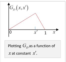
However, a little thought about the original differential equation makes it clear.

As a function of $x$ for given $x^{\prime },$  away from the point $x^{\prime },G_D\left(x,x^{\prime }\right)$ must be just a straight line: the solution of $d^{2}f/d{x}^2=0.$ 

$G_D\left(x,x^{\prime }\right)$ goes to zero at the boundaries $x=0,x=1$ and has unit discontinuity in slope at $x=x^{\prime }.$  (Differentiating a slope discontinuity gives a step discontinuity, the next differentiation gives the delta function.)

The neat way to write it is in terms of

$$x_{<}=\min \left(x,x^{\prime }\right),x_{>}=\max \left(x,x^{\prime }\right),$$

In terms of these variables, the expression is simple:

$$G_D\left(x,x^{\prime }\right)=x_{<}\left(1-x_{>}\right).$$

Exercise:  Convince yourself that this is correct, in particular the change in slope, and that it is symmetric in $x,x^{\prime },$ as a Green’s function must be.

For three-dimensional problems, we’ll often find it best to use the complete set of states representation for angle-type variables, the direct integration for radial variables.

Two Different Representations of the Green’s Function

It’s worth thinking a little more about the two different expressions for the Green’s function.

A:     $G_D\left(x,x^{\prime }\right)=2{\displaystyle \sum _n\frac{\sin n\pi x\sin n\pi x^{\prime }}{{\pi }^2{n}^2}},$

B:    $G_D\left(x,x^{\prime }\right)=x_{<}\left(1-x_{>}\right).$

Expression A is a sum over all eigenstates of the differential operator, to be expected since it comes from integrating the delta function, which, being infinitely sharp, has contributions from all momentum/energy states. And, it’s difficult to visualize.

Expression B apparently involves only zero energy eigenstates of the operator: one satisfying the $x=0$ boundary condition, the other the  $x=1$ boundary condition, and, in contrast to A, is very easy to see.  But how can these two expressions be equivalent? The point is that B has a slope discontinuity, this generates the delta function when the differential operator is applied, and it means that if you take a Fourier transform of B as a function of $x$ for fixed $x^{\prime },$ there will be contributions from all energies.

These two representations are a recurring theme (especially in homework questions).

Physics

Does this one-dimensional model have any electrostatic realization?  Yes$—$it’s equivalent to an infinite uniform sheet of charge between two infinite parallel grounded conductors, which will have negative charge induced, to give linear potential drop from the charged sheet to the plates.

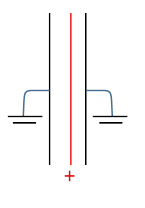
Exercise: for a non-central sheet of charge, what are the charges induced? 

A mechanical one-dimensional realization would be a taut string pushed out of line by a sharp object to a V shape (in general with different length arms, of course). The two-dimensional generalization would be a rubber sheet attached to, say, the four sides of a square frame, pushed up at one point.  Everywhere else the rubber would relax to the minimum energy, which is given by the displacement $z$ (in linear approximation) satisfying the two-dimensional ${\nabla }^{2}z=0.$ 

Point Charge Inside a Grounded Cubical Box: Induced Surface Charge

The obvious three-dimensional generalization of the one-dimensional delta function presented above to a 3D box with the six walls at $x,y,z=0,1,$ is

$\begin{array}{l}\delta \left(\overrightarrow{r}-{\overrightarrow{r}}^{\prime }\right)=\delta \left(x-x^{\prime }\right)\delta \left(y-y^{\prime }\right)\delta \left(z-z^{\prime }\right)\\ =8{\displaystyle \sum _{n,m,\ell }\sin n\pi x\sin n\pi x^{\prime }\sin m\pi y\sin m\pi y^{\prime }}\sin \ell \pi z\sin \ell \pi z^{\prime }.\end{array}$

Using the same argument as that above for the one-dimensional case, the three-dimensional Dirichlet Green’s function inside a cubical box with all walls at zero potential is:

$G_D\left(\overrightarrow{r},{\overrightarrow{r}}^{\prime }\right)=8{\displaystyle \sum _{n,m,\ell }\frac{\sin n\pi x\sin n\pi x^{\prime }\sin m\pi y\sin m\pi y^{\prime }\sin \ell \pi z\sin \ell \pi z^{\prime }}{{\pi }^2\left(n^2+m^2+{\ell }^2\right)}}.$

It’s straightforward to check that

${\nabla }^2{G}_D\left(\overrightarrow{r},{\overrightarrow{r}}^{\prime }\right)=-\delta \left(\overrightarrow{r}-{\overrightarrow{r}}^{\prime }\right).$

So what can we do with this Green’s function?  Well, if we put a charge at any point $\left(x,y,z\right)$ inside a grounded conducting cubical box, this gives the potential at any other point $\left(x^{\prime },y^{\prime },z^{\prime }\right)$ and, in particular, by differentiating this expression in the normal direction at the walls, we can find the charge induced on the walls (remember they’re held at zero potential, meaning grounded, so charge will flow into these walls when the point charge is put inside the box). 

For example, the surface charge density induced at the point  $\left(x^{\prime },y^{\prime },1\right)$ on the top face is

$\sigma \left(x^{\prime },y^{\prime }\right)=8{\displaystyle \sum _{n,m,\ell }\frac{\ell \sin n\pi x\sin m\pi y\sin \ell \pi z\sin n\pi x^{\prime }\sin m\pi y^{\prime }\cos \ell \pi }{\pi \left(n^2+m^2+{\ell }^2\right)}}.$

Potential Inside a Cubical (Nonconducting) Box with Given Potential at Walls

Recall now one of the results of the Reciprocation Theorem: a point charge at $\overrightarrow{r}$ inside a closed  grounded container induces a surface charge density $\sigma \left({\overrightarrow{r}}^{\prime }\right)$: from the theorem, if we have an identical empty container with specified potentials $\phi \left({\overrightarrow{r}}^{\prime }\right)$ at the walls (so it’s not in general a connected conductor), the potential at the corresponding point $\overrightarrow{r}$ inside

$\phi \left(\overrightarrow{r}\right)={\epsilon }_0{\displaystyle \underset{S}{\int }\phi \left({\overrightarrow{r}}^{\prime }\right)}\sigma \left({\overrightarrow{r}}^{\prime }\right)da={\epsilon }_0{\displaystyle \underset{S}{\int }\phi \left({\overrightarrow{r}}^{\prime }\right)}\frac{\partial G_D\left(\overrightarrow{r},{\overrightarrow{r}}^{\prime }\right)}{\partial n}da.$

We can take five of the six walls to be at zero potential, then use linearity to add six such results.

Assume the potential is  $\phi \left(x^{\prime },y^{\prime }\right)$ on the face at $z=1,$ so $0\le x^{\prime },y^{\prime }<1,$ and $\phi =0$ on the other faces. Then at any point inside the cube,

$\begin{array}{c}\phi \left(\overrightarrow{r}\right)={\epsilon }_0{\displaystyle \underset{S}{\int }\phi \left({\overrightarrow{r}}^{\prime }\right)}\sigma \left({\overrightarrow{r}}^{\prime }\right)da={\epsilon }_0{\displaystyle \underset{S}{\int }\phi \left({\overrightarrow{r}}^{\prime }\right)}\frac{\partial G_D\left(\overrightarrow{r},{\overrightarrow{r}}^{\prime }\right)}{\partial n}da\\ =8{\epsilon }_0{\displaystyle \underset{\text{top face}}{\int }\phi \left(x^{\prime },y^{\prime }\right)}{\displaystyle \sum _{n,m,\ell }\frac{\ell \sin n\pi x\sin m\pi y\sin \ell \pi z\sin n\pi x^{\prime }\sin m\pi y^{\prime }\cos \ell \pi }{\pi \left(n^2+m^2+{\ell }^2\right)}}d{x}^{\prime }d{y}^{\prime }.\end{array}$

In the next lecture, we will analyze this same problem with a rather different approach, and find a different-looking (but of course equivalent) answer. In fact, the two approaches are equivalent to the two forms of the Green's function discussed earlier in this lecture for the simple one-dimensional system.

Exercise:  Suppose the six faces of a cube are conductors, but insulated from each other. Suppose the top face is held at potential $V,$ the others are grounded. Use the Reciprocation Theorem to prove the potential at the center of the cube is $V/6.$ Does this approach also work for a dodecahedron?

previous  index  next