13. Math Reminder: Simple Functions in the Complex Plane

    Michael Fowler, UVa

Finding Solutions to Laplace’s Equation

It is an amazing fact that when we take the functions we’ve known since childhood (well, almost):

$$f\left(x\right)=x^2,\sqrt{x},\log x,\sin x,\dots$$

and just replace the real variable $x$ by a complex one $z=x+iy,$ to give a complex function, call it $w\left(z\right),$ of the complex variable $z,$

$$w\left(z\right)=w\left(x,y\right)=u\left(x,y\right)+iv\left(x,y\right),$$

the (real) functions $u\left(x,y\right),v\left(x,y\right)$ satisfy Laplace’s equation in the $\left(x,y\right)$ plane!

That is,

$${\nabla }^{2}u\left(x,y\right)=0,{\nabla }^{2}v\left(x,y\right)=0.$$

 These are solutions in search of a problem….

To see how they might be used, consider the simplest function in the list:

$$z^2={\left(x+iy\right)}^2=\left(x^2-y^2\right)+i\left(2xy\right).$$

 The two functions are

$$u\left(x,y\right)=x^2-y^2,v\left(x,y\right)=2xy.$$

 It’s easy to check that they do indeed satisfy the 2D Laplace equation, so, to pick one, $v\left(x,y\right)$ could be an electrostatic potential.  Let’s plot equipotentials to see where it might be relevant:

$$\phi \left(x,y\right)=2xy=\text{constant}\text{.}$$

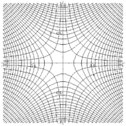
For a positive constant, this is a family of rectangular hyperbolae covering for positive constant the ++ and $–$ sectors of the plane, for negative constant the other two sectors.

Notice this function is zero on the axes, so it describes the potential near a corner where two conducting sheets meet at right angles. For example, this would be a good approximation near one corner inside a rectangular pipe (like a waveguide).

Exercise: show equipotentials for $u\left(x,y\right),$ describe them in words, then state how they relate to those for $v\left(x,y\right).$

But why do these functions generate potentials in the 2D complex plane?

The reason is simple: they are differentiable: that means there is a well-defined function

$$w^{\prime }\left(z\right)=\frac{dw}{dz}={\lim }_{\Delta z\to 0}\frac{w\left(z+\Delta z\right)-w\left(z\right)}{\Delta z}.$$

Why is differentiability such a powerful statement? After all, for a real variable, being differentiable merely means (loosely speaking) being a well-behaved continuous function.  Yet in the two dimensions of a complex variable, it clearly means so much more$—$the separate real and imaginary parts must obey these Laplacian equations! The crucial difference from the real case is that in the complex plane $\Delta z\to 0$ can happen in different ways: you could choose to approach the origin along the real axis or along the imaginary axis, and both must give the same result, or, by definition, the function isn’t differentiable.

That is, for $w=u+iv$ with $u\left(z\right),v\left(z\right)$ real functions, and $z=x+iy,$

$$\frac{\partial w\left(x+iy\right)}{\partial x}=\frac{\partial w\left(x+iy\right)}{\partial \left(iy\right)},$$

or, spelling it out,

$$\frac{\partial u\left(x,y\right)}{\partial x}+i\frac{\partial v\left(x,y\right)}{\partial x}=\frac{\partial u\left(x,y\right)}{\partial \left(iy\right)}+i\frac{\partial v\left(x,y\right)}{\partial \left(iy\right)}.$$

 

Now equating real and imaginary parts,

$$\frac{\partial u}{\partial x}=\frac{\partial v}{\partial y},\frac{\partial v}{\partial x}=-\frac{\partial u}{\partial y},$$

 

and from this is follows that

$$\frac{{\partial }^{2}u\left(x,y\right)}{\partial x^2}+\frac{{\partial }^{2}u\left(x,y\right)}{\partial y^2}=0,$$

 

that is,

$${\nabla }^{2}u\left(x,y\right)=0,{\nabla }^{2}v\left(x,y\right)=0.$$

 

Furthermore, again of course in two dimensions, for

$$\overrightarrow{\nabla }u=\left(\frac{\partial u}{\partial x},\frac{\partial u}{\partial y}\right),\text{we have }\overrightarrow{\nabla }u\cdot \overrightarrow{\nabla }v=0,$$

 

meaning that if we take the potential  $\phi \left(x,y\right)=u\left(x,y\right)$ then the lines of constant $v\left(x,y\right)$ are everywhere perpendicular to the $u\left(x,y\right)$ equipotentials, that is, the $v\left(x,y\right)$ equipotentials are the $u\left(x,y\right)$ field lines (and vice versa): their direction at each point is that of the local electric field.  For example, the diagram above plots the equipotentials of $u\left(x,y\right)$ and $v\left(x,y\right)$ for the function $w\left(z\right)=z^2.$

Singularities

The definition of differentiation above can be used to show that

$$\frac{d}{dz}\left(\frac{1}{z}\right)=-\frac{1}{z^2},$$

 

just as for a real variable, so the function $1/z$ can be differentiated everywhere in the complex plane except at the origin.  The singularity at the origin is termed a “pole”, for obvious reasons.

Other Singularities: Cuts, Sheets, etc.

Poles are of course not the only possible singularities. For example, $\ln z$ has a singularity at the origin.  Now, $\ln z=\ln r{e}^{i\theta }=\ln r+i\theta .$ The infinite value at the origin is from the $\ln r$ term, but notice that if we go around the unit circle, $\theta$ increases by $2\pi ,$ and if we go around again it increases by a further $2\pi .$ This means that the value of $\ln z$ is not uniquely defined: any given point in the complex plane has values differing by $2\pi ni,n$ any integer.  This is handled by replacing the single complex plane with a pile of sheets, and a cut going out from the origin. To find $\ln z,$ you need to know not only $z,$ but also which sheet you’re on: going up one sheet means $\ln z$ has increased by $2\pi i.$ When you cross the cut, you go to the next sheet, like a multilevel parking garage. 

The cut can go out from the origin in any direction, the standard arrangement is along the real axis, either positive or negative.

The square root function similarly has a cut, but only two sheets.

The above is quoted from my Quantum Mechanics lectures, where there are further details, including contour integration, which we’ll need later in this course.

In electrostatics problems, usually we don’t venture on to other sheets$—$the cut can correspond in position to a physical charged plane, we’ll see some examples. (In other areas of physics, singularities on other sheets can be important: for example, in quantum scattering theory, a resonance corresponds to a pole on a “nonphysical” sheet, and sometimes increasing a coupling constant can bring the pole on to the physical sheet, where it becomes a bound state.)

In the following lectures, we’ll see how familiarity with the properties of some simple functions in the complex plane can lead to quick solutions of some Jackson 2D electrostatics problems.