previous  index  next 

23. Field of a Charged Conducting Disc

    Michael Fowler, UVa

Charge Density on the Disc

This is a classic problem, solved in the early nineteenth century by Green (and is Jackson problem 3.3!)  It turns out that the capacitance of a disc of radius $a$ is $C=8{\epsilon }_{0}a.$  A sphere of radius $a$ has capacitance $4\pi {\epsilon }_{0}a$, a factor $\pi /2$ greater.  Cavendish measured the ratio sphere/disc experimentally as 1.57, probably in the 1770's.  Very impressive.

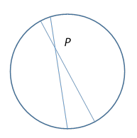
Your first thought might be: doesn't the charge all migrate to the edge, just as charge in a solid goes to the surface? The answer is no$—$and it's worth thinking about why not. Consider first a uniformly charged sphere. Pick an arbitrary point P inside (but not the center$—$that's obviously trivial). We know there's no field, but how exactly does the cancellation from all the surface elements work? Take one element of surface, subtending a narrow cone at P, and continue the lines of the cone through P to trace out another surface element on the opposite side.  These two surface elements won't have the same area: they subtend the same solid angle at P, so their areas are in the ratios of the squares of their distances from P.  But the electrostatic field at P goes as the inverse square of the distance, so the two forces exactly balance.

Now back to the disc: it's got circular symmetry, but if the charge is around the edge, this cancellation no longer works, because the corresponding small segments of the circle scale linearly with distance from an interior point, but the inverse square law of force still holds, so the nearer charge is more important.  In other words, if we start with a large number of equal charges arranged equally spaced around the edge, then move one of them inwards and allow those still on the edge to rearrange slightly to restore equal spacing, the one moved inwards will move further away from the edge, towards the middle. Evidently, if all the charges are free to move, the equilibrium arrangement will have a nonzero density over the whole disc.  

OK, so what about the charge distribution on the disc?   Finding the field is Jackson problem 3.3, but Jackson takes the charge density as given.  Zangwill says there is no truly simple way to calculate it.  I beg to differ$—$Purcell gives the simple explanation presented below, but Kelvin was almost certainly aware of it a century earlier.

Here’s the analysis: we’re looking for an (obviously circularly symmetric) charge distribution such that everywhere on the disc the electric field has zero horizontal (plane of the disc) component.  Otherwise, it's not electrostatics. We know, of course, the field will have a vertical component, opposite on the two sides, proportional to the charge density.  

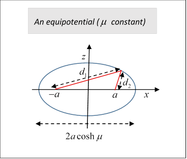
The key is to think about the argument for a uniformly charged sphere.  Zangwill actually states at the end of his analysis (based on taking the disc as the limiting case of an oblate ellipsoid, that the charge distribution equals the projection of a uniformly charged hemisphere onto its equatorial plane.  This is the clue!

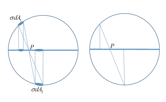
On the uniformly (surface) charged sphere, the forces from the two elements of charge $\sigma d{A}_1,\sigma d{A}_2$ as felt at P are equal and opposite, as we've argued. But now suppose we project those charges on to the equatorial plane (see figure). The ratio of their distances from P is unaltered, as is clear from the second diagram. Therefore, the forces from them at P are still equal and opposite. Doing this for the entire sphere, we see that a disc with charge density equal to that projected to the equatorial plane from a uniformly charged sphere will generate zero electric field parallel to the disc, and so will be in electrostatic equilibrium.

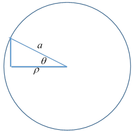
So what is the charge distribution?  We use $\rho$ for the radial variable on the disc, following standard cylindrical coordinate notation.

The ratio of the projected surface area to the area on the sphere is $\sin \theta =\sqrt{a^2-{\rho }^2}/a,$ so the appropriate charge density on the disc is proportional to the inverse of this.  The integral to get the total charge $Q$ is simple, the result is a surface charge density on the disc

$$\sigma \left(\rho \right)=\frac{Q}{2\pi a\sqrt{a^2-{\rho }^2}}.$$

Finding the Field

Jackson's (problem 3.3) suggested method of solution, using spherical harmonics, is a bad idea, for reasons that will become evident. 

The good news is that the problem can be solved in elegant fashion using oblate spheroidal coordinates (a nineteenth century favorite) and the correct solution makes clear why ordinary spherical harmonics lead to difficulties.  You can get the first part, the distant potential, correctly with ordinary spherical harmonics (as suggested by Jackson), but you cannot match it to a solution close to the disc.  The reason is simple. To match the angular spherical harmonics, you must match an odd power of distance outside to an even power inside. However, the correct solution of the problem is an odd power of distance along the $z\text{-}$ axis at all distances. The potential has a singularity at the edge of the disc, so the usual matching conditions at the crucial radius $a$ are invalid. There are ways around this: the inner region can be broken into two, above and below the disc, with separate expansions in each, either even or odd Legendre polynomials form a complete set if restricted to half the angular range.  This is correct, but technically difficult and not very transparent.  Several “solutions” posted on the web are simply wrong.

(Note: If you’re not familiar with oblate spherical harmonics, you can get comfortable with them in less time that you’ll otherwise spend on this Jackson problem.)

Oblate Spherical Harmonics

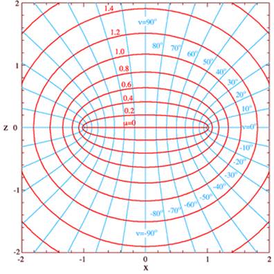
The natural way to solve this problem is to use oblate spheroidal harmonics $\left(\mu ,\nu ,\phi \right).$   This becomes evident on looking at the lines of constant $\mu$ in the coordinate diagram here (from Wikipedia).  They look just like the equipotentials we would intuitively expect from a charged disc, and in particular the $\mu =0$ line corresponds to a thin disc in 3D, just what we expect for a conductor.  Of course, we haven’t proved anything yet!  To prove our guess correct, we need to establish that there is some function of $\mu$ only which satisfies the three-dimensional ${\nabla }^2\phi =0$ everywhere except at $\mu =0.$

The coordinates look like this in cross section, in three dimensions they are rotationally symmetric about the central line $\nu =\pi /2.$ 

The Cartesian coordinates are:

$\begin{array}{l}x=a\cosh \mu \cos \nu \cos \varphi ,\\ y=a\cosh \mu \cos \nu \sin \varphi ,\\ z=a\sinh \mu \sin \nu .\end{array}$

(This is not as bad as it looks: the azimuthal $\varphi$ dependence is trivial, from the corresponding rotational symmetry, so we're left with, essentially, a function of $\rho =\sqrt{x^2+y^2}$ and $z.$ We have to be careful with signs, though, since $\rho$ is defined as positive, so to get the right picture it's better to plot an $xz$ cross section as shown above.

 

(In this cross section$—$azimuthal $\varphi =0$ $—$the equations are equivalent to a complex variable equation, $x+iz=\cosh \left(\mu +i\nu \right),$ using the addition formula for cosh, recall these were the equipotentials we found in 2D for a charged strip. In that 2D case, the potential was simply $\mu .$ That can’t be the case here, though, because ${\nabla }^2$ is different.) 

The constant $\mu$ surfaces are ellipsoids (here oblate spheroids):

$$\frac{x^2+y^2}{{\cosh }^2\mu }+\frac{z^2}{{\sinh }^2\mu }=a^2.$$

Note from the figure that we take $0\le \mu <\infty .$

This is often written in cylindrical coordinates, corresponding to a constant $\phi$ surface:  

$$\frac{{\rho }^2}{{\cosh }^2\mu }+\frac{z^2}{{\sinh }^2\mu }=a^2.$$

The foci of all the ellipses are at $a,-a,$ the ellipses are said to be "confocal". The lengths of the major and minor axes are $2a\cosh \mu ,2a\sinh \mu$ respectively.

Constant $\nu$ surfaces are:

$$\frac{{\rho }^2}{{\cos }^2\nu }-\frac{z^2}{{\sin }^2\nu }=a^2.$$

A tricky point: we parametrize the whole plane with positive $\mu ,$ so from $z=a\sinh \mu \sin \nu ,$ $\nu$ has the same sign as $z.$ Therefore these surfaces are half-hyperbolas, divided at $z=0,$ with foci also at $a,-a,$ and they are field lines. That is, $\nu$ is discontinuous at $\mu =0,$ across the (infinitely thin) disc. (In the next lecture, we look at the field for a hole in a charged conducting sheet. We can use the same coordinate system, but must change the parametrization so that the discontinuity only happens across the charged sheet, the opposite situation to the disc.)

Recalling that the definition of an ellipse is that the sum of its distances from two points (the foci) is a constant (in fact the length of the major axis), and for a hyperbola the difference is constant (also the length of its major axis, but be careful with our notation, in most places the lengths of these major axes are $2a,$ but in these coordinates, $2a$ is the distance between the foci).

We define the (always positive!) distances (switching now from $\rho z$ to just the $xz$ plane) by

$d_1^2={\left(x+a\right)}^2+z^2,d_2^2={\left(x-a\right)}^2+z^2.$

It follows that

$$\cosh \mu =\frac{d_1+d_2}{2a}\cos \nu =\frac{d_1-d_2}{2a}.$$

(The equipotential ellipse major axis has length $2a\cosh \mu$.)  We can also see from this that the curves cut at right angles (think of moving incrementally so that the sum/difference from two fixed points is constant). 

Electrostatics of a Charged Conducting Disc

Obviously, from the pictures, the natural choice for potential is some function of the coordinate $\mu .$ 

So we need to solve ${\nabla }^2\Phi =0$ for this spheroidal system, that is (Wikipedia):

$\begin{array}{l}{\nabla }^2\Phi =\\ \frac{1}{a^2\left({\sinh }^2\mu +{\sin }^2\nu \right)}\left[\frac{1}{\cosh \mu }\frac{\partial }{\partial \mu }\left(\cosh \mu \frac{\partial \Phi }{\partial \mu }\right)+\frac{1}{\cos \nu }\frac{\partial }{\partial \nu }\left(\cos \nu \frac{\partial \Phi }{\partial \nu }\right)\right]+\frac{1}{a^2{\cosh }^2\mu {\cos }^2\nu }\frac{{\partial }^2\Phi }{\partial {\varphi }^2}\\ =0.\end{array}$

But, thankfully, we are looking for a potential that is a function of $\mu$ only, that is, a solution of:

$$\frac{\partial }{\partial \mu }\left(\cosh \mu \frac{\partial \Phi }{\partial \mu }\right)=0,\text{ so }\frac{\partial \Phi }{\partial \mu }=\frac{\text{const}\text{.}}{\cosh \mu }$$

The solution is (with $\Phi ={\Phi }_0\text{ at }\mu =0$ )

$$\Phi \left(\mu \right)={\Phi }_0\left(1-\frac{2}{\pi }\arctan \sinh \mu \right)=\frac{2}{\pi }{\Phi }_0\arcsin \frac{1}{\cosh \mu }.$$

Now

$$\cosh \mu =\frac{\sqrt{{\left(\rho +a\right)}^2+z^2}+\sqrt{{\left(\rho -a\right)}^2+z^2}}{2a}$$

So on the $z\text{-}$ axis,

$$\Phi \left(\mu \right)=\frac{2}{\pi }{\Phi }_0\arcsin \frac{a}{\sqrt{a^2+z^2}}=\frac{2}{\pi }{\Phi }_0\arctan \frac{a}{\left|z\right|}.$$

And, for the far region $z>a$, we can use the standard expansion, to get

$\arctan (a/z)=a/z-\frac{{\left(a/z\right)}^3}{3}+\frac{{\left(a/z\right)}^5}{5}-\frac{{\left(a/z\right)}^7}{7}+\cdots ={\displaystyle \sum _{n=0}^{\infty }\frac{{(-1)}^n{\left(a/z\right)}^{2n+1}}{2n+1}};z\ge a,$

and this agrees with Jackson’s result for $z>a.$ 

For $z<a,$ obviously the series diverges, but we can just use

$\arctan \left(a/z\right)=\pi /2-\arctan \left(z/a\right).$

Therefore, our solution for the potential along the $z\text{-}$ axis is

$\begin{array}{c}\Phi \left(\mu \right)=\frac{2}{\pi }{\Phi }_0\arctan \frac{a}{\left|z\right|}\\ =\frac{2}{\pi }{\Phi }_0{\displaystyle \sum _{n=0}^{\infty }\frac{{(-1)}^n{\left(a/z\right)}^{2n+1}}{2n+1}},z\ge a,\\ ={\Phi }_0-\frac{2}{\pi }{\Phi }_0{\displaystyle \sum _{n=0}^{\infty }\frac{{(-1)}^n{\left(z/a\right)}^{2n+1}}{2n+1}},0\le z\le a.\end{array}$

Notice we can't get this result by matching Legendre polynomial expansions at $r=a,$ because $z^{-\left(2n+1\right)}$ would have to match with $z^{2n}.$ 

This is just on the axis, of course: let’s check that our expression for the potential is in fact constant over the whole disc in the $\left(x,y\right)$ plane.  We have

$$\Phi \left(\mu \right)=\frac{2}{\pi }{\Phi }_0\arcsin \frac{1}{\cosh \mu }=\frac{2}{\pi }{\Phi }_0\arcsin \frac{2a}{\sqrt{{\left(\rho +a\right)}^2+z^2}+\sqrt{{\left(\rho -a\right)}^2+z^2}}.$$

We know that the equipotentials are ellipsoids (here oblate spheroids), and this is clear from the formula, remembering that an ellipse is defined as the set of curves such that the sum of distances from two fixed points, the foci, is constant.  This is exactly what we see in the denominator.  The foci are all at $a,-a.$ The flat disc itself is a degenerate ellipsoid, with foci of a cross section, such as the $xz$ plane, coinciding with the ends of the major axis.  Therefore, the denominator is the sum of distances from the two ends, and for a point on the disc, that's just $2a.$ This establishes that the potential is indeed constant on the disc.  (Note: at least one online "solution" takes positive square roots for $z=0$ in this expression, so gets the denominator equal to $2\rho ,$ which is nonsense.)

Exercise:  For $z=0$ but outside the disc, the potential is nonzero, it's worth looking at it for small distances away from the disc, but in the plane.

 Charge Density on Disc from Potential

The charge density is of course proportional to the strength of the perpendicular electric field strength.

The potential near the origin on the $z\text{-}$axis is ${\Phi }_0-\frac{2}{\pi }{\Phi }_0\frac{z}{a},$ so the field strength is $2{\Phi }_0/\pi a.$ 

To find the normal field strength, hence the charge density, at other points on the disc, consider an equipotential very close to the plate, in cross section an ellipse with major semi-axis we can take to be $a$ and minor semi-axis $b\ll a.$ 

Then the equation of the ellipse is very close to  $\frac{{\rho }^2}{a^2}+\frac{z^2}{b^{{}^2}}=1,$ and in particular the height of the equipotential above the disc at distance $\rho$ from the center is $z=\left(b/a\right)\sqrt{a^2-{\rho }^2}.$ 

Taking an equipotential sufficiently close, the field strength must vary across the disc as the inverse of the distance between this equipotential and the (equipotential) disc, that is, it must be

$$E\left(\rho \right)=\frac{2{\Phi }_0}{\pi \sqrt{a^2-{\rho }^2}},$$

 and the charge density is 

$$\sigma \left(\rho \right)=\frac{4{\epsilon }_0{\Phi }_0}{\pi \sqrt{a^2-{\rho }^2}},$$

confirming the argument at the beginning of the lecture.

The total charge is therefore

$Q={\displaystyle \underset{0}{\overset{a}{\int }}2\pi \rho \sigma \left(\rho \right)d\rho }={\displaystyle \underset{0}{\overset{a}{\int }}2\pi \rho \frac{4{\epsilon }_0{\Phi }_0}{\pi \sqrt{a^2-{\rho }^2}}d\rho }=8{\epsilon }_0{\Phi }_0{\displaystyle \underset{0}{\overset{a}{\int }}\frac{\rho }{\sqrt{a^2-{\rho }^2}}d\rho }=8{\epsilon }_0{\Phi }_{0}a.$ 

A sphere of radius $a$ has capacitance $4\pi {\epsilon }_{0}a$, a factor $\pi /2$ greater. 

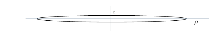
What About a Disc of Finite Thickness?

Glancing at the long thin ellipse pictured above, it’s at least plausible that the capacitance of a disc of thickness $2b$ would be well approximated by that of this ellipsoid.  Assuming $b\ll a,$ the potential along the $z$ axis

$\Phi \left(z=b\right)\cong {\Phi }_0\left(1-\frac{2}{\pi }\frac{b}{a}\right).$

Think about the electric field lines emanating from charge $Q$ on the infinitely thin disc. They all pass through this thin ellipsoid too, and beyond it are identical from that same charge actually on the ellipsoid. But the potential on the ellipsoid is down by the factor in the equation above, so it follows that the capacitance of the ellipsoid is increased by the inverse, to leading order:

$C_b\cong 8{\epsilon }_{0}a\left(1+\frac{2}{\pi }\frac{b}{a}\right).$

In fact, a lot of work has been done on this problem, using a more accurate shape for the disc (a thin cylinder, like a coin) beginning with Maxwell in 1877.  Even Thomson (Lord Kelvin) found Maxwell’s paper hard to follow, so we won’t try.  A more accessible presentation has been given by Kirk McDonald (online) updated in 2019, carefully analyzing charge distribution on a coin-like cylinder.  For the infinitely thin disc case as discussed above, the charge density diverges as the inverse square root of distance from the edge, but for the thin cylinder there are upper and lower edges, and a cylindrical surface between, and the charge density near those edges diverges only as the inverse cube root of distance.  (This follows from our earlier 2D discussion of charge near corners.)  A reasonable assumption is that this cube root behavior prevails for distances from the edge of order the thickness, but away from that the charge distribution is as for the infinitely thin disc.  Taking the crossover to be at $b,$ and matching the charge densities there, McDonald finds the charge on the cylindrical surface makes a big enough contribution that the finite thickness correction becomes of order $\sqrt{b/a}$ rather than $b/a.$ For details, see his paper.

previous  index  next