49  Propagation in the Ionosphere, Whistlers

    Michael Fowler, UVa

Jackson 7.6

Discovery of the Ionosphere: Plasma Reflection of Radio Waves

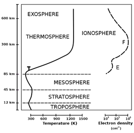
The first attempts at communication using radio waves were carried out in the late 1890’s by Gulielmo  Marconi, mostly in England. In 1901, he succeeded is transmitting radio waves across the Atlantic, after having been assured by physicists that this couldn’t happen because radio waves, like light, travel in straight lines. His success was thanks to the ionosphere, a series of ionized layers from approximately 50 km height up to 1000 km height, with a maximum at around 300 kilometers.

The ionization is caused by ultraviolet solar radiation: the ionosphere has a maximum free electron density of order 10¹⁰$—$10¹² electrons/m³ at a height around 300km. (Higher up the atmosphere is thinner, further down the free electrons are rapidly recaptured.) There is a large day/night variation (at least a factor of 5), and further variation from changing solar activity.

This layer of ionization is a plasma, so the methods developed in the previous lecture can be used to understand wave reflection.  

Recalling from the previous lecture that the wave impedance in a plasma

$$Z_{\text{pl}}=Z_0\frac{\omega }{\sqrt{{\omega }^2-{\omega }_{\text{pl}}^2}},$$

and ${\omega }_{\text{pl}}^2=n_e{e}^2/{\epsilon }_{0}m.$ 

On going up from the Earth’s surface, where $n_e=0,$ as the free electron density climbs from zero to the maximum 10¹⁰$—$10¹² the plasma frequency goes up from zero to a value in the range 6 to 60 MHz.

Radio waves sent upwards with frequency $\omega$ less than this will be reflected at the height where the local plasma frequency matches the wave frequency $\omega ={\omega }_{\text{pl}},$ so the impedance $Z_{\text{pl}}$ becomes infinite.  Higher frequency waves $\omega >{\omega }_{\text{pl}}$ will continue out into space.  

A more precise analysis gives essentially the same result: provided the electron density varies slowly on the plasma wavelength scale, a WKB solution to the wave equation works, except close to the critical height where reflection takes place, but there an Airy function is an excellent approximation, exactly as for a Schrödinger wave function at the edge of a bound state.  For details of these techniques, see my quantum mechanics notes.

Effect of the Earth’s Magnetic Field

Perhaps surprisingly, the Earth’s magnetic field plays a crucial role in the reflection, essentially because the natural circular motion of an electron in this field happens to be at a frequency of the same order of magnitude as the relevant plasma frequencies.  

For a simple model of the field’s effects, we take a plasma in a constant magnetic field ${\overrightarrow{B}}_0$  in the (vertical) $z$ -direction, and send straight upwards a wave with electric field $\overrightarrow{E}{e}^{-i\omega t}$, so the vector $\overrightarrow{E}$ lies in the $\left(x,y\right)$ plane, spanned by unit vectors $\widehat{\overrightarrow{x}},\widehat{\overrightarrow{y}}.$  

Note: This is just a simple model! The real world is more complicated, the ionosphere has layers that vary from day to night, and with sunspot activity. Radio signals can go up at an angle, and be refracted. Nevertheless, this simple model contains a lot of the essential physics, and is well worth studying.

Taking the magnetic field of the wave itself to be negligible compared with the fixed field ${\overrightarrow{B}}_0,$ the equation of motion of an electron in the wave’s electric field plus the Earth’s magnetic field will be

$$m\ddot{\overrightarrow{r}}-e{\overrightarrow{B}}_0\times \dot{\overrightarrow{r}}=-e\overrightarrow{E}{e}^{-i\omega t}.$$

Electron Motion in Electric Field from Wave

First, we’ll analyze the motion without ${\overrightarrow{B}}_0.$

Usually we would express the wave electric field as a sum of components linearly polarized in the $\widehat{\overrightarrow{x}}$ and $\widehat{\overrightarrow{y}}$ directions, but for this problem, since the magnetic field generates circular motion, it turns out to be more natural to take as the basis waves that are circularly polarized, meaning electric fields

$$\overrightarrow{E}{e}^{-i\omega t}=\left(\widehat{\overrightarrow{x}}\pm i\widehat{\overrightarrow{y}}\right)E\left(\cos \omega t-i\sin \omega t\right),$$

so the actual physical electric field is

$$\mathrm{Re}\left(\overrightarrow{E}{e}^{-i\omega t}\right)=\widehat{\overrightarrow{x}}E\cos \omega t\pm \widehat{\overrightarrow{y}}E\sin \omega t,$$

that is, field vectors of constant magnitude circling at angular speed $\omega ,$ anticlockwise or clockwise $\left(\pm \omega \right)$ about $\widehat{\overrightarrow{z}}.$  (Linear polarization is then just a sum of equal amplitude circular waves rotating in opposite directions.)

A steady state solution of the electron equation of motion,

$$m\ddot{\overrightarrow{r}}=-e\overrightarrow{E}{e}^{-i\omega t},$$

is for the electron to circle in the $\left(x,y\right)$ plane, its position vector $\overrightarrow{r}$ parallel to $\overrightarrow{E},$ the electric field providing the centripetal force, so

$$mr{\omega }^2=eE$$

(the electronic charge taken as $-e.$ )  We could add a constant velocity in the direction of the field.

Electron Motion in Wave Field Plus Earth’s Magnetic Field

If we now add in the external magnetic field ${\overrightarrow{B}}_0$ term, for the steady circular motion the velocity vector $\dot{\overrightarrow{r}}$ is in the $\left(x,y\right)$ plane, perpendicular to the position vector $\overrightarrow{r}$ and having magnitude $\omega r,$ so ${\overrightarrow{B}}_0\times \dot{\overrightarrow{r}}$ is in the radial direction, with length $B_0\omega r,$ inwards or outwards depending on rotation direction.

The centripetal equation then becomes

$$mr{\omega }^2\pm e{B}_0\omega =eE,$$

the sign of $\omega$ depending on the direction of rotation, and writing ${\omega }_B=e{B}_0/m,$ we have

$$\overrightarrow{r}=\frac{e}{m\omega \left(\omega \mp {\omega }_B\right)}\overrightarrow{E},$$

the electron following the rotating field in a circle with radius proportional to the field strength.  (This ${\omega }_B$ is sometimes written ${\omega }_c$ for cyclotron frequency.)

The physics is that when the magnetic field ${\overrightarrow{B}}_0$ is added, there is an additional radial force $e\overrightarrow{v}\times {\overrightarrow{B}}_0$ on the electron, its sign depending on that of $\overrightarrow{v},$ so if the net central force is stronger for right circularly polarized light, it will be weaker for left polarization, and the radius of the orbit changes to adjust the centripetal acceleration $mr{\omega }^2$ to balance.

The equation of motion is still satisfied if we add a constant velocity in the perpendicular ( $\widehat{\overrightarrow{z}}$ ) direction, so the typical motion is a spiral path around a magnetic field line.  The direction of the rotation is called the helicity, positive helicity (negative sign in equation) corresponding to left-handed optical circular polarization according to Jackson, but unfortunately there doesn’t seem to be a uniform convention on labeling these rotation directions, so be careful.  

Permittivity of the Ionosphere in a Circular Polarized Basis

The ionosphere is, as the name implies, a partially ionized gas, so the permittivity is that of a plasma. Without the magnetic field, as we found earlier, it would be $\epsilon \left(\omega \right)/{\epsilon }_0=1-\left({\omega }_{\text{pl}}^2/{\omega }^2\right).$

However, as we established in the previous section, with the external magnetic field present, the dipole response$—$position of the electron$—$changes to $\overrightarrow{r}=e\overrightarrow{E}/m\omega \left(\omega \mp {\omega }_B\right),$ so the permittivity is different depending on the rotation direction:

$$\frac{{\epsilon }_{\mp }}{{\epsilon }_0}=1-\frac{{\omega }_{\text{pl}}^2}{\omega \left(\omega \mp {\omega }_B\right)}.$$

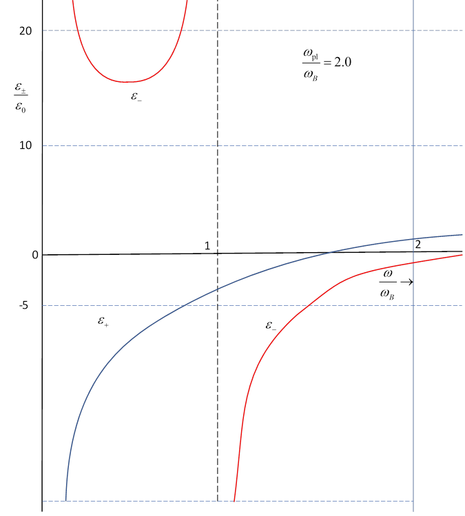
Jackson presents (page 218) two graphs of these functions for values ${\omega }_{\text{pl}}/{\omega }_B=2.0,0.5$ and here they are: it is instructive to look over them at the same time: ${\epsilon }_{\pm }$ are plotted as functions of $\omega /{\omega }_B.$ (By the way, these are sketches, not mathematically precise.)

Beginning at high wave frequency, obviously ${\epsilon }_{\pm }\cong {\epsilon }_0$ for $\omega \gg {\omega }_{\text{pl}},{\omega }_B.$

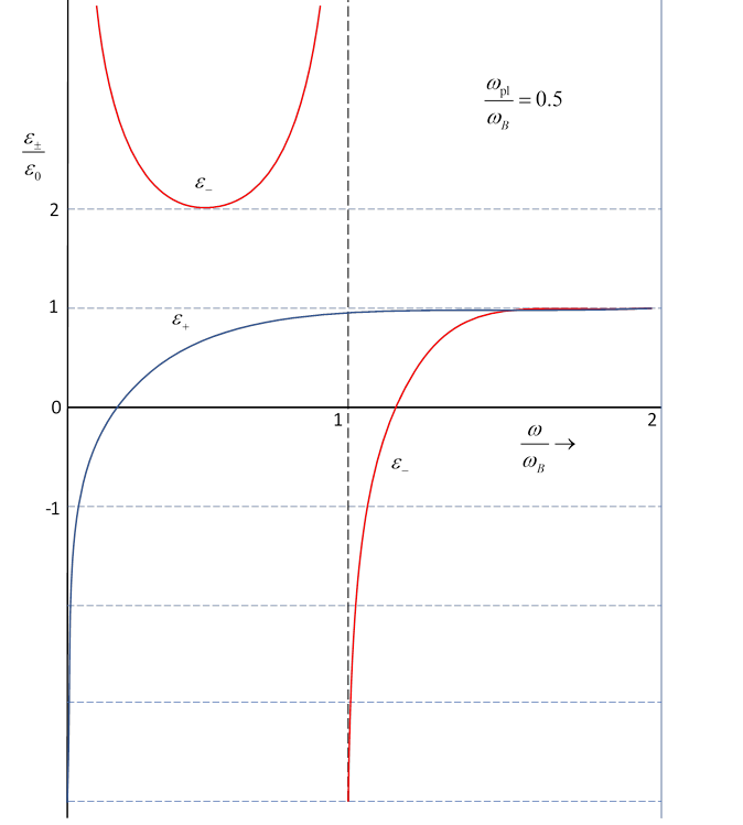
Looking first at the curve for ${\epsilon }_{+},$ going down in frequency, ${\epsilon }_{+}$ goes to zero (look at the formula, then the graphs) when $\omega \left(\omega +{\omega }_B\right)={\omega }_{\text{pl}}^2,$ the wave will be reflected.  

 

For lower frequencies, the wave will also be reflected, with exponentially decaying penetration into the plasma, $E^{\prime }\left(z\right)=E^{\prime }\left(0\right)e^{-z/\delta },\delta =c/\sqrt{{\omega }_{\text{pl}}^2-\omega \left(\omega +{\omega }_B\right)}.$

 As discussed in the previous lecture, no energy is lost here on reflection, but there is a phase shift.

It should be mentioned though, that for very low frequencies, such as the old “long wave” radio transmissions, some energy is absorbed in the ionosphere, because the electron-ion collision time can no longer be neglected compared with oscillation time. 

The curve for ${\epsilon }_{-}$ is more interesting. It not only goes negative on lowering the frequency from a high value, it goes to minus infinity at a nonzero frequency$—$so the penetration depth goes to zero.  What’s going on? We see from the expression for ${\epsilon }_{\mp }\left(\omega \right)$ that this occurs at $\omega ={\omega }_B,$ the cyclotron frequency. This means the rotating electric field is in sync with the natural circular motion of the electron in the external magnetic field, in fact we have a cyclotron$—$the electric field accelerates the electron, which spirals out to larger circular orbits at the same frequency, but of course higher speed, so energy is absorbed. The function of a complex variable ${\epsilon }_{-}\left(z\right)$ has a pole on the real axis. (If we think of the basis states of a 2D SHO as chiral modes, this can be viewed as half a SHO!)

Below $\omega ={\omega }_B,$ ${\epsilon }_{-}\left(\omega \right)$ is positive, so waves will propagate through the plasma. Notice from the graphs that there are regions where ${\epsilon }_{-},{\epsilon }_{+}$ have opposite signs, so only one helicity will propagate, and an incoming wave will have its polarization changed.

Whistlers

As $\omega \to 0,$ ${\epsilon }_{-}\left(\omega \right)\to {\epsilon }_0{\omega }_{\text{pl}}^2/\omega {\omega }_B,$ so the phase velocity $v=1/\sqrt{\mu \epsilon }\to c\sqrt{\omega {\omega }_B}/{\omega }_{\text{pl}}.$ From $\omega =vk,$

$\omega =ck\sqrt{\omega {\omega }_B}/{\omega }_{\text{pl}},$ so $\omega =c^2{k}^2{\omega }_B/{\omega }_{\text{pl}}^2$ and the group velocity

$$\begin{array}{c}{v}_g\left(\omega \right)=d\omega /dk=2c^{2}k{\omega }_B/{\omega }_{\text{pl}}^2\\ =2c/{\omega }_{\text{pl}}\left(ck{\omega }_B/{\omega }_{\text{pl}}\right)=2c\sqrt{{\omega }_B\omega }/{\omega }_{\text{pl}}.\end{array}$$

Looking at the graph for positive ${\epsilon }_{-}\left(\omega \right)$ at low $\omega ,$ consider the frequencies corresponding to sound, say 1KHz. Taking ${\omega }_B$ =1MHz and ${\omega }_{\text{pl}}$ =10MHz (these are reasonable handwaving estimates) gives $v_g$ for sound frequencies to be of order of 10^-1 $–$10^-2c.

This analysis turns out to be the solution of a mystery sound found in radio communications during the First World War: an initially high-pitched audio note that rapidly decreased in frequency over a period of several seconds, and dubbed a “whistler”.  Notice in the above equation that the group velocity decreases with frequency.

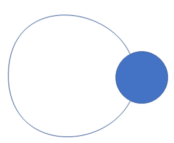
A flash of lightning sends a powerful electromagnetic pulse up towards the ionosphere, including low frequency ${\epsilon }_{-}$ waves which are not reflected. The initial pulse contains many frequencies, and so rapidly spreads out along its path, which is upwards. The Earth’s (dipole) magnetic field lines guide the wave (we haven’t shown a proof of this, but it is correct), and the signal returns to Earth in the other hemisphere (see diagram) where it can be reflected back, and detected. The path length is of order 10⁵ kilometers, well outside the ionosphere, and whistler observations established the existence of the plasmasphere, a thin plasma at a height of several earth radii.  

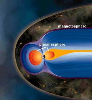
 Historical Footnote: Notice in the picture the much larger magnetosphere$—$the region where the Earth’s magnetic field determines the motion of the charged particles. Outside this is the solar wind, a constant stream of particles from the Sun. The magnetosphere protects the Earth (therefore us) by deflecting these particles. The overall shape of the magnetosphere, and the nature of the solar wind during sunspot activity, were much clarified by Joan Feynman, who showed interest in science as a young girl, but was discouraged by her mother and grandmother, who assured her that the female brain was not able to understand such things. Luckily, her older brother Dick told her that was all nonsense. Among many other achievements, her analysis of radiation from the solar wind entering the magnetosphere led to important changes in spacecraft design.

Faraday Rotation, Pulsars and Deep Space Plasma

Since the phase velocity $v=1/\sqrt{\mu \epsilon },$ in the presence of the magnetic field the two circular polarizations have different phase velocities, so a linearly polarized wave (a sum of opposite circularly polarized waves) will have its plane of polarization rotating as it propagates.  

This is called the Faraday effect, or Faraday rotation, and predated Maxwell’s realization of the electromagnetic nature of light.  Faraday argued that the rotation strongly suggested some relation between light and magnetism.

Faraday rotation plays an important role in astronomy. Pulsars emit blips of radiation, covering a range of frequencies, and are linearly polarized. The signals reach us after traversing large distances in very dilute plasma, in general with low magnetic fields present. We can find the total Faraday rotation by integrating the incremental rotation along the path, it will depend on the local plasma density and the magnetic field component in the direction of the path.  It also depends$—$crucially$—$on the wavelength, going as ${\lambda }^2.$ This enables us to separate out the different frequency components, and yields much information about plasma densities and magnetic field strengths in deep space.  See Jackson problem 7.15, and Wikipedia.

previous  index  next