57 Radiating Systems, Multipole Fields and Radiation

    Michael Fowler, UVa

Introduction

In this lecture, we'll analyze the electromagnetic fields radiated by a compact time-varying charge and current distribution.  The radiated field amplitudes decay with distance as $1/r.$ The charges and currents also have "near field" contributions going as $1/r^2,$ essentially the time-dependent version of the fields from static charges and steady currents, but here we'll only consider the far (radiated) fields.

(Note: In fact, the $1/r^2$ fields are relevant in the radiation zone (far away) for one thing: analyzing radiated angular momentum (which we’re not going to do here).  A $1/r^2$ component in the direction of radiation will couple with a perpendicular component to give a Poynting vector perpendicular to the direction of radiation, but the angular momentum radiated has a factor $r$ from $\overrightarrow{r}\times \overrightarrow{p}$.)

The three relevant length scales are the size of the generating distribution, call it $d,$ a typical wavelength of the radiation, say $\lambda ,$ and the distance at which we're detecting the radiation, say $r.$  We'll always assume $r\gg \lambda ,d.$ 

Since the problem is linear, it is enough to solve it for a single frequency of oscillation.  As we shall see, that greatly simplifies the analysis.  So (in the next section) we’ll take

$\rho \left(\overrightarrow{r},t\right)=\rho \left(\overrightarrow{r}\right)e^{-i\omega t},\overrightarrow{J}\left(\overrightarrow{r},t\right)=\overrightarrow{J}\left(\overrightarrow{r}\right)e^{-i\omega t}.$ 

But first, a brief review of the basic Green’s function we need (repeating to some extent material from lecture 39, hopefully worth refreshing at this point).

Formal Solution of the Wave Equations: the Green’s Function

Recall that in the Lorenz gauge

$\overrightarrow{\nabla }\cdot \overrightarrow{A}+\frac{1}{c^2}\frac{\partial \phi }{\partial t}=0,$

the equations for the scalar and vector potentials generated by a charge and current distribution are

$\begin{array}{l}{\nabla }^2\phi -\frac{1}{c^2}\frac{{\partial }^2\phi }{\partial t^2}=-\rho /{\epsilon }_0,\\ {\nabla }^2\overrightarrow{A}-\frac{1}{c^2}\frac{{\partial }^2\overrightarrow{A}}{\partial t^2}=-{\mu }_0\overrightarrow{j}.\end{array}$

To get the full picture of potentials generated by time-dependent charge and current distributions, we need the Green’s function with a delta function source in both space and time:

$\left({\nabla }^2-\frac{1}{c^2}\frac{{\partial }^2}{\partial t^2}\right)G\left(\overrightarrow{r},t;{\overrightarrow{r}}^{\prime },t^{\prime }\right)=-4\pi \delta \left(\overrightarrow{r}-{\overrightarrow{r}}^{\prime }\right)\delta \left(t-t^{\prime }\right).$

This is, with $R=\left|\overrightarrow{r}-{\overrightarrow{r}}^{\prime }\right|,$ 

$G^{\left(\pm \right)}\left(R,t-t^{\prime }\right)=\frac{1}{2\pi }{\displaystyle \underset{-\infty }{\overset{\infty }{\int }}\frac{e^{\pm ikR-i\omega \left(t-t^{\prime }\right)}}{4\pi R}}d\omega ,k=\omega /c,$

and the integral over $\omega$ is just the delta function in time, that is,

$G^{\left(\pm \right)}\left(R,t-t^{\prime }\right)=\frac{1}{R}\delta \left(\left(t-t^{\prime }\right)\mp \frac{R}{c}\right).$

The choice $G^{\left(+\right)}\left(R,t-t^{\prime }\right)=\frac{1}{R}\delta \left(\left(t-t^{\prime }\right)-\frac{R}{c}\right)$ is the retarded Green’s function.  It's geometrically equivalent to the expanding spherical pulse going radially outward from a flash of light at point ${\overrightarrow{r}}^{\prime }$ at time $t^{\prime }.$ 

Solving ${\nabla }^2\phi -\frac{1}{c^2}\frac{{\partial }^2\phi }{\partial t^2}=-\rho /{\epsilon }_0$ with this Green’s function:

$\phi \left(\overrightarrow{r},t\right)=\frac{1}{{\epsilon }_0}{\displaystyle \int d{\overrightarrow{r}}^{\prime }d{t}^{\prime }{G}^{\left(+\right)}\left(\overrightarrow{r},t;{\overrightarrow{r}}^{\prime },t^{\prime }\right)\rho \left({\overrightarrow{r}}^{\prime },t^{\prime }\right)}$

that is,

$\phi \left(\overrightarrow{r},t\right)=\frac{1}{4\pi {\epsilon }_0}{\displaystyle \int d{\overrightarrow{r}}^{\prime }\frac{1}{\left|\overrightarrow{r}-{\overrightarrow{r}}^{\prime }\right|}}\rho {\left({\overrightarrow{r}}^{\prime },t^{\prime }\right)}_{\text{ret}}$

where the “ret” for retarded means measuring $\rho \left({\overrightarrow{r}}^{\prime }\right)$ at the (earlier) time $t^{\prime }$ at which a light signal emitted from ${\overrightarrow{r}}^{\prime }$ would reach $\overrightarrow{r}$ at $t.$

Similarly,

${\nabla }^2\overrightarrow{A}-\frac{1}{c^2}\frac{{\partial }^2\overrightarrow{A}}{\partial t^2}=-{\mu }_0\overrightarrow{j}$ 

has solution

$\overrightarrow{A}\left(\overrightarrow{r},t\right)=\frac{{\mu }_0}{4\pi }{\displaystyle \int d^3{r}^{\prime }\frac{{\left[\overrightarrow{J}\left({\overrightarrow{r}}^{\prime },t^{\prime }\right)\right]}_{\text{ret}}}{\left|\overrightarrow{r}-{\overrightarrow{r}}^{\prime }\right|}}=\frac{{\mu }_0}{4\pi }{\displaystyle \int d^3{r}^{\prime }\frac{\overrightarrow{J}\left({\overrightarrow{r}}^{\prime },t-\frac{\left|\overrightarrow{r}-{\overrightarrow{r}}^{\prime }\right|}{c}\right)}{\left|\overrightarrow{r}-{\overrightarrow{r}}^{\prime }\right|}}$

Radiation at a Single Frequency

In general, these equations are difficult to solve (see lecture 39), because we need to know the detailed development of the current distribution at each point since we're adding the contributions with the time delay, and that varies from point to point. However, if the whole distribution is oscillating at the same frequency, all that's changing in time is the phase, and the phase of the signal from any point is just given by the distance from that point to the observer.

That is, for

$\overrightarrow{J}\left(\overrightarrow{r},t\right)=\overrightarrow{J}\left(\overrightarrow{r}\right)e^{-i\omega t}$ 

the phase delay is just $\omega \left(t-t^{\prime }\right)=k\left|\overrightarrow{r}-{\overrightarrow{r}}^{\prime }\right|,$ and writing $\overrightarrow{A}\left(\overrightarrow{r},t\right)=\overrightarrow{A}\left(\overrightarrow{r}\right)e^{-i\omega t},$ 

$\overrightarrow{A}\left(\overrightarrow{r}\right)=\frac{{\mu }_0}{4\pi }{\displaystyle \int \overrightarrow{J}\left({\overrightarrow{r}}^{\prime }\right)\frac{e^{ik\left|\overrightarrow{r}-{\overrightarrow{r}}^{\prime }\right|}}{\left|\overrightarrow{r}-{\overrightarrow{r}}^{\prime }\right|}{d}^3{r}^{\prime }},\omega =ck.$ 

Furthermore, the vector potential is all we need in the radiation zone: we can drop $\phi ,$ since the magnetic field is given by $\overrightarrow{H}=\left(1/{\mu }_0\right)\overrightarrow{\nabla }\times \overrightarrow{A},$ and the electric field is $\left(i{Z}_0/k\right)\overrightarrow{\nabla }\times \overrightarrow{H}$ with $Z_0=\sqrt{{\mu }_0/{\epsilon }_0}.$ 

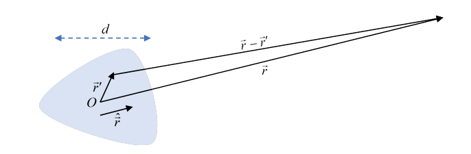
Taking the origin to be in the compact region of currents and sources (shaded in above figure), for $r\gg d,$ from the figure,

$\left|\overrightarrow{r}-{\overrightarrow{r}}^{\prime }\right|\cong r-\widehat{\overrightarrow{r}}\cdot {\overrightarrow{r}}^{\prime }$ 

so

$\underset{kr\to \infty }{\lim }\overrightarrow{A}\left(\overrightarrow{r}\right)=\frac{{\mu }_0}{4\pi }\frac{e^{ikr}}{r}{\displaystyle \int \overrightarrow{J}\left({\overrightarrow{r}}^{\prime }\right)e^{-ik\widehat{\overrightarrow{r}}\cdot {\overrightarrow{r}}^{\prime }}{d}^3{r}^{\prime }}.$ 

(We've replaces $\left|\overrightarrow{r}-{\overrightarrow{r}}^{\prime }\right|$ by $r$ in the denominator, a good approximation provided $r\gg d,$  but we can't neglect the phase factor $ik\widehat{\overrightarrow{r}}\cdot {\overrightarrow{r}}^{\prime }$ except in the case $\left|k{r}^{\prime }\right|\ll 1,$ the wavelength much greater than the dimensions of the oscillating current, and we don't want to impose that extra restriction here.)

The natural way to approach the problem systematically is to expand the exponential:

$\underset{kr\to \infty }{\lim }\overrightarrow{A}\left(\overrightarrow{r}\right)=\frac{{\mu }_0}{4\pi }\frac{e^{ikr}}{r}{\displaystyle \sum _n\frac{{\left(-ik\right)}^n}{n!}}{\displaystyle \int \overrightarrow{J}\left({\overrightarrow{r}}^{\prime }\right){\left(\widehat{\overrightarrow{r}}\cdot {\overrightarrow{r}}^{\prime }\right)}^n{d}^3{r}^{\prime }}.$ 

The Leading Term: Electric Dipole

The radiation is in general dominated by the first term in the exponential expansion (although symmetries could make this term zero):

${\overrightarrow{A}}_{\text{el dip}}\left(\overrightarrow{r}\right)=\frac{{\mu }_0}{4\pi }\frac{e^{ikr}}{r}{\displaystyle \int \overrightarrow{J}\left({\overrightarrow{r}}^{\prime }\right)d^3{r}^{\prime }}.$ 

(Remember all this has an understood $e^{-i\omega t}.$ It's like doing the time-independent Schrodinger equation.)

This is called the "electric dipole term".  Obviously, it's only nonzero if at some instant in time there is a net current in some direction, but then half a cycle later, it will be flowing the other way, so the charge is sloshing backwards and forwards.  But that's what happens in an oscillating dipole$—$and it's easy the see they're mathematically equivalent:

${\displaystyle \int \overrightarrow{J}{d}^3{r}^{\prime }}=-{\displaystyle \int {\overrightarrow{r}}^{\prime }\left({\overrightarrow{\nabla }}^{\prime }\cdot \overrightarrow{J}\right)d^3{r}^{\prime }=-i\omega {\displaystyle \int {\overrightarrow{r}}^{\prime }\rho \left({\overrightarrow{r}}^{\prime }\right)d^{3}r}}=-i\omega \overrightarrow{p}.$ 

where we used an integration by parts of the three separate vector components, followed by using $\overrightarrow{\nabla }\cdot \overrightarrow{J}=i\omega \rho .$ Remember all terms have time dependence $e^{-i\omega t},$ so the current and dipole are out of phase by $\pi /2,$ as a simple picture of oscillating charge suggests.

In terms of the dipole, then, the radiation vector potential  

${\overrightarrow{A}}_{\text{el dip}}\left(\overrightarrow{r},t\right)=-\frac{i{\mu }_0\omega }{4\pi }\overrightarrow{p}\frac{e^{ikr-i\omega t}}{r},\overrightarrow{p}={\displaystyle \int {\overrightarrow{r}}^{\prime }\rho \left({\overrightarrow{r}}^{\prime }\right)d^3{r}^{\prime }}.$ 

The fields follow from $\overrightarrow{H}=\left(1/{\mu }_0\right)\overrightarrow{\nabla }\times \overrightarrow{A},$  $\overrightarrow{E}=\left(i{Z}_0/k\right)\overrightarrow{\nabla }\times \overrightarrow{H}$ with $Z_0=\sqrt{{\mu }_0/{\epsilon }_0}$ (this is the impedance of the vacuum, about 377 ohms. See the discussion of waveguide impedance in the previous lecture). 

The $\overrightarrow{\nabla }\times$ only operates on the factor $e^{ikr}/r,$ and we drop the $1/r^2$ (near field) term, giving

${\overrightarrow{H}}_{\text{el dip}}=\frac{c{k}^2}{4\pi }\left(\widehat{\overrightarrow{r}}\times \overrightarrow{p}\right)\frac{e^{ikr-i\omega t}}{r},{\overrightarrow{E}}_{\text{el dip}}=Z_0{\overrightarrow{H}}_{\text{el dip}}\times \widehat{\overrightarrow{r}}=-\frac{k^2}{4\pi {\epsilon }_0}\frac{e^{ikr-i\omega t}}{r}\widehat{\overrightarrow{r}}\times \left(\widehat{\overrightarrow{r}}\times \overrightarrow{p}\right).$ 

Exercise:  draw a sketch!  $\overrightarrow{A}$ is always parallel to the dipole, so $\overrightarrow{H}$ must be azimuthal, and $\overrightarrow{E}$ is perpendicular to $\overrightarrow{H},\overrightarrow{r}.$

The time averaged power per solid angle

$\begin{array}{c}\frac{d{P}_{\text{el dip}}}{d\Omega }=\frac{1}{2}\mathrm{Re}\left[r^2\widehat{\overrightarrow{r}}\cdot \overrightarrow{E}\times {\overrightarrow{H}}^{\ast }\right]\\ =\frac{c^2{Z}_0}{32{\pi }^2}{k}^4{p}^2{\sin }^2\theta .\end{array}$ 

(Remember $\overrightarrow{E},\overrightarrow{H}$ are both going down as $1/r.$ )

The total power is (using $\overline{{\sin }^2\theta }=2/3,{\displaystyle \int d\Omega =4\pi }$ )

$P_{\text{el dip}}=\frac{c^2{Z}_0}{12\pi }{k}^4{p}^2=\frac{Z_0}{12\pi c^2}{\omega }^4{p}^2=\frac{{\mu }_0}{12\pi c}{\omega }^4{p}^2.$ 

Notice this goes as the fourth power of the frequency!

Landau's Treatment of Dipole Radiation from a Very Compact Charge Distribution

Landau (Classical Theory of Fields, 4^th edition, page 189) discusses the case of a radiating dipole charge distribution small in size compared to the wavelength of the radiation, so

${\overrightarrow{A}}_{\text{el dip}}\left(\overrightarrow{r},t\right)=\frac{{\mu }_0}{4\pi r}{\displaystyle \int \overrightarrow{J}\left({\overrightarrow{r}}^{\prime },t^{\prime }\right)d^3{r}^{\prime }}$ 

and here we take $t^{\prime }=t-r/c$ independent of ${\overrightarrow{r}}^{\prime }.$ 

We can sum over the charges in this system and write (following Landau, we use dots for time differentiation)

${\overrightarrow{A}}_{\text{el dip}}\left(\overrightarrow{r},t\right)=\frac{{\mu }_0}{4\pi r}{\displaystyle \sum e\overrightarrow{v}}=\frac{{\mu }_0}{4\pi r}\frac{d}{dt}{\displaystyle \sum e\overrightarrow{r}=\frac{{\mu }_0\dot{\overrightarrow{p}}}{4\pi r}}.$ 

Now we need to find $\overrightarrow{B}=\overrightarrow{\nabla }\times \overrightarrow{A}.$ Here Landau exploits the fact that in the radiation zone, at some instant in time, $\overrightarrow{A}\left(\overrightarrow{r},t\right)$ only varies in the $\widehat{\overrightarrow{r}}$ direction, it’s a function of $r,$ so we have $\overrightarrow{B}=\widehat{\overrightarrow{r}}\times {\overrightarrow{\nabla }}_r\overrightarrow{A}.$  (Check this!) Furthermore, in fact $\overrightarrow{A}$ only depends on $r$ in the combination $t-r/c,$ so $\partial /\partial r$ is equivalent to $-\left(1/c\right)\partial /\partial t.$ Visualize the wave moving outwards to see how this can be.

So $\overrightarrow{B}=\left(1/c\right)\dot{\overrightarrow{A}}\times \widehat{\overrightarrow{r}}$ and

$\overrightarrow{H}=\frac{1}{4\pi rc}\ddot{\overrightarrow{p}}\times \widehat{\overrightarrow{r}}.$

This is a general result$—$it is not at this point restricted to single frequency motion (but it does depend on the charge distribution size being small compared with the wavelength).  The magnetic field only depends on the instantaneous acceleration of the dipole at the appropriate earlier time.  As before, from Maxwell’s equations ${\overrightarrow{E}}_{\text{el dip}}=Z_0{\overrightarrow{H}}_{\text{el dip}}\times \widehat{\overrightarrow{r}},$ and the differential instantaneous radiation intensity

$dI=\frac{{\mu }_0}{16{\pi }^{2}c}{\ddot{\overrightarrow{p}}}^2{\sin }^2\theta .$ 

(This differs by a factor of two from the formula in the last section, that was an average for an oscillating field, this is the momentary intensity.)

The total power on integrating over solid angle is

$P=\frac{{\mu }_0}{6\pi c}{\ddot{\overrightarrow{p}}}^2.$ 

Radiation from an Accelerating Particle

From the formula above, we can immediately find the power emitted by a single accelerating particle: imagine the dipole to consist of a fixed charge and a close by, but moving, opposite charge at $\overrightarrow{r},$ so $\overrightarrow{p}=q\overrightarrow{r}.$ Then writing the acceleration of the moving charge $\ddot{\overrightarrow{r}}=\overrightarrow{a},$ we have

$$P=\frac{{\mu }_0}{6\pi c}{q}^2{\overrightarrow{a}}^2.$$ 

This is called the Larmor formula.  We’ll discuss the important relativistic generalization later in the course.

A Simple Dipole Example: Short Center-Fed Linear Antenna

Note that Jackson's example here is a short antenna, $d\ll \lambda .$ This means that the charge distribution on each branch can be taken to be uniform, since the charge distribution equilibrates almost at the speed of light. (Not completely obvious, but true.)

For discussion and animations of a dipole antenna both receiving and transmitting,  click here.  Note that in this lecture, following Jackson, we are in the short dipole approximation. 

Taking the antenna along the $z$ axis, the origin at its center, the current is the real part of

         $$J_z=\delta \left(x\right)\delta \left(y\right)e^{-i\omega t}\left(1-\frac{2\left|z\right|}{d}\right)I_0.$$ 

Charge conservation ensures the linear current decrease,

$-i\omega \rho \left(\overrightarrow{r}\right)e^{-i\omega t}=-\overrightarrow{\nabla }\cdot \overrightarrow{J}=I_0\delta \left(x\right)\delta \left(y\right)e^{-i\omega t}\left(2/d\right)\mathrm{sgn}z.$ 

Hence the dipole moment

$\begin{array}{c}\overrightarrow{p}={\displaystyle \int {\overrightarrow{r}}^{\prime }\rho \left({\overrightarrow{r}}^{\prime }\right)d^3{r}^{\prime }}=\widehat{\overrightarrow{z}}{\displaystyle \underset{-d/2}{\overset{d/2}{\int }}\frac{2I_0}{-i\omega d}{z}^{\prime }d{z}^{\prime }}\\ =\widehat{\overrightarrow{z}}\left(\frac{2I_0}{-i\omega d}\right)2\cdot \frac{1}{2}{\left(\frac{d}{2}\right)}^2=\widehat{\overrightarrow{z}}\left(\frac{2i{I}_{0}d}{2\omega }\right).\end{array}$ 

The total power radiated from a short center-fed linear dipole antenna is therefore

$$P=\frac{Z_0{I}_0^2{\left(kd\right)}^2}{48\pi }=\frac{Z_0{I}_0^2{d}^2}{48\pi c^2}{\omega }^2.$$ 

Recalling that we just found for an oscillating dipole of strength $p$ the radiation went as ${\omega }^4$, this result is at first glance surprising.  The point is that here there is a fixed input current, not a fixed dipole strength.  From the charge conservation equation, at higher frequencies, meaning faster movement of the charge in the wires, less charge is needed to get the same current, so the dipole strength is down by a factor $1/\omega .$  

The power produced in a DC resistance is $P=\frac{1}{2}{I}^{2}R.$  Analogously, the radiation resistance of an antenna is defined as

$$R_{\text{rad}}=\frac{P}{\frac{1}{2}{I}_0^2}=\frac{Z_0{d}^2}{24\pi c^2}{\omega }^2.$$ 

The Next Order Term:  Magnetic Dipole and Electric Quadrupole Radiation

The next term in the expansion is

$\overrightarrow{A}\left(\overrightarrow{r}\right)=\frac{{\mu }_0}{4\pi }\frac{e^{ikr}}{r}\left(\frac{1}{r}-ik\right){\displaystyle \int \overrightarrow{J}\left({\overrightarrow{r}}^{\prime }\right)\left(\widehat{\overrightarrow{r}}\cdot {\overrightarrow{r}}^{\prime }\right)d^3{r}^{\prime }}.$ 

(but we'll drop the higher order $1/r$ term in the bracket).

Using the vector identity

$\left({\overrightarrow{r}}^{\prime }\times \overrightarrow{J}\right)\times \widehat{\overrightarrow{r}}=\overrightarrow{J}\left(\widehat{\overrightarrow{r}}\cdot {\overrightarrow{r}}^{\prime }\right)-{\overrightarrow{r}}^{\prime }\left(\overrightarrow{J}\cdot \widehat{\overrightarrow{r}}\right)$ 

we can write the integrand as a sum of parts symmetric and antisymmetric in $\overrightarrow{J},{\overrightarrow{r}}^{\prime }$: 

$\overrightarrow{J}\left({\overrightarrow{r}}^{\prime }\right)\left(\widehat{\overrightarrow{r}}\cdot {\overrightarrow{r}}^{\prime }\right)=\frac{1}{2}\left[\overrightarrow{J}\left({\overrightarrow{r}}^{\prime }\right)\left(\widehat{\overrightarrow{r}}\cdot {\overrightarrow{r}}^{\prime }\right)+{\overrightarrow{r}}^{\prime }\left(\widehat{\overrightarrow{r}}\cdot \overrightarrow{J}\left({\overrightarrow{r}}^{\prime }\right)\right)\right]+\frac{1}{2}\left({\overrightarrow{r}}^{\prime }\times \overrightarrow{J}\left({\overrightarrow{r}}^{\prime }\right)\right)\times \widehat{\overrightarrow{r}}.$ 

Following Jackson, we'll begin with the second term, the antisymmetric part, which turns out to be

Magnetic Dipole Radiation

You may recall from magnetostatics that the magnetic moment from a current in a loop of wire is

$\overrightarrow{m}=\frac{1}{2}I{\displaystyle \oint \overrightarrow{r}\times d\overrightarrow{\ell }}=\frac{1}{2}{\displaystyle \oint \overrightarrow{r}\times d\overrightarrow{J}},$ 

and the natural generalization to a continuum current distribution is

$\overrightarrow{m}=\frac{1}{2}{\displaystyle \int {\overrightarrow{r}}^{\prime }\times \overrightarrow{J}\left({\overrightarrow{r}}^{\prime }\right)d^3{r}^{\prime }}.$ 

(In terms of particles, this would be $\overrightarrow{m}=\frac{1}{2}{\displaystyle \sum {\overrightarrow{r}}_j\times q_j{\overrightarrow{v}}_j}.$ )

Comparing with the equation for $\overrightarrow{A}\left(\overrightarrow{r},t\right)$ above, we see the antisymmetric current distribution contributes

${\overrightarrow{A}}_{\text{mag dip}}\left(\overrightarrow{r},t\right)=-\frac{{\mu }_0}{4\pi }\frac{ik{e}^{i\left(kr-\omega t\right)}}{r}\overrightarrow{m}\times \widehat{\overrightarrow{r}}$ .

This is magnetic dipole radiation.  The magnetic field (to leading order) is

${\overrightarrow{H}}_{\text{mag dip}}=\frac{k^2}{4\pi }\frac{e^{i\left(kr-\omega t\right)}}{r}\left(\widehat{\overrightarrow{r}}\times \overrightarrow{m}\right)\times \widehat{\overrightarrow{r}}.$ 

Exercise: Verify this.

Comparing Electric Dipole and Magnetic Dipole Fields

Recall now that the magnetic field from an electric dipole was ${\overrightarrow{H}}_{\text{el dip}}=\frac{c{k}^2}{4\pi }\left(\widehat{\overrightarrow{r}}\times \overrightarrow{p}\right)\frac{e^{ikr-i\omega t}}{r},$ and the electric field from an electric dipole is ${\overrightarrow{E}}_{\text{el dip}}=Z_0\overrightarrow{H}\times \widehat{\overrightarrow{r}}=-\frac{k^2}{4\pi {\epsilon }_0}\frac{e^{ikr-i\omega t}}{r}\widehat{\overrightarrow{r}}\times \left(\widehat{\overrightarrow{r}}\times \overrightarrow{p}\right).$

So the electric dipole radiation and the magnetic dipole radiation are essentially duals of each other, the electric and magnetic fields being swapped.  Of course, the units are different, and there's a sign difference in the corresponding Maxwell equations, so to get from the electric dipole to the magnetic takes 

$\overrightarrow{E}\to Z_0\overrightarrow{H},Z_0\overrightarrow{H}\to -\overrightarrow{E},\overrightarrow{p}\to \overrightarrow{m}/c.$ 

The angular power distribution in magnetic dipole radiation is precisely that from an electric dipole, losing the factor $c^2$ to correct for the different units of electric and magnetic dipoles,

$\frac{d{P}_{\text{mag dip}}}{d\Omega }=\frac{Z_0}{32{\pi }^2}{k}^4{m}^2{\sin }^2\theta .$ 

The total power, using $\overline{{\sin }^2\theta }=2/3$ and total angle is $4\pi ,$ is

$P_{\text{mag dip}}=\frac{Z_0}{12\pi }{k}^4{m}^2.$ 

Electric Quadrupole Radiation

Returning to the equation

$\overrightarrow{J}\left({\overrightarrow{r}}^{\prime }\right)\left(\widehat{\overrightarrow{r}}\cdot {\overrightarrow{r}}^{\prime }\right)=\frac{1}{2}\left[\overrightarrow{J}\left({\overrightarrow{r}}^{\prime }\right)\left(\widehat{\overrightarrow{r}}\cdot {\overrightarrow{r}}^{\prime }\right)+{\overrightarrow{r}}^{\prime }\left(\widehat{\overrightarrow{r}}\cdot \overrightarrow{J}\left({\overrightarrow{r}}^{\prime }\right)\right)\right]+\frac{1}{2}\left({\overrightarrow{r}}^{\prime }\times \overrightarrow{J}\left({\overrightarrow{r}}^{\prime }\right)\right)\times \widehat{\overrightarrow{r}},$

we’ll now focus on the part symmetric in$\overrightarrow{J},{\overrightarrow{r}}^{\prime }$, the first term.

With 20-20 hindsight, we use the following identity:

${\displaystyle \sum _{\gamma }\frac{\partial }{\partial {r^{\prime }}_{\gamma }}}\left({r^{\prime }}_{\alpha }{r^{\prime }}_{\beta }{J}_{\gamma }\right)=J_{\alpha }{r^{\prime }}_{\beta }+J_{\beta }{r^{\prime }}_{\alpha }+{r^{\prime }}_{\alpha }{r^{\prime }}_{\beta }{\displaystyle \sum _{\gamma }\frac{\partial J_{\gamma }}{\partial {r^{\prime }}_{\gamma }}}.$ 

Since the current distribution is compact, on integrating over all of space the left-hand side is zero.

Then taking the dot product of the result with the constant unit vector ${\widehat{r}}_{\beta }$ gives

${\displaystyle \int \left[\left(\widehat{\overrightarrow{r}}\cdot {\overrightarrow{r}}^{\prime }\right)\overrightarrow{J}+\left(\widehat{\overrightarrow{r}}\cdot \overrightarrow{J}\right){\overrightarrow{r}}^{\prime }\right]}{d}^3{r}^{\prime }=-{\displaystyle \int {\overrightarrow{r}}^{\prime }\left(\widehat{\overrightarrow{r}}\cdot {\overrightarrow{r}}^{\prime }\right){\overrightarrow{\nabla }}^{\prime }\cdot \overrightarrow{J}\left({\overrightarrow{r}}^{\prime }\right)}.$ 

This is the symmetric function we need.

Using charge conservation ${\overrightarrow{\nabla }}^{\prime }\cdot \overrightarrow{J}\left({\overrightarrow{r}}^{\prime }\right)=i\omega \rho \left({\overrightarrow{r}}^{\prime }\right),$ this symmetric part gives rise to the vector potential (in the radiation zone, dropping $1/r^2$ terms)

${\overrightarrow{A}}_{\text{el quad}}\left(\overrightarrow{r}\right)=-\frac{{\mu }_{0}c{k}^2}{8\pi }\frac{e^{ikr}}{r}{\displaystyle \int {\overrightarrow{r}}^{\prime }\left(\widehat{\overrightarrow{r}}\cdot {\overrightarrow{r}}^{\prime }\right)\rho \left({\overrightarrow{r}}^{\prime }\right)d^3{r}^{\prime }.}$

The fields in the radiation zone are

${\overrightarrow{H}}_{\text{el quad}}=ik\widehat{\overrightarrow{r}}\times {\overrightarrow{A}}_{\text{el quad}}/{\mu }_0,{\overrightarrow{E}}_{\text{el quad}}=ik{Z}_0\left(\widehat{\overrightarrow{r}}\times {\overrightarrow{A}}_{\text{el quad}}\right)\times \overrightarrow{r}/{\mu }_0$ 

so

${\overrightarrow{H}}_{\text{el quad}}\left(\overrightarrow{r}\right)=-\frac{ic{k}^3}{8\pi }\frac{e^{ikr}}{r}{\displaystyle \int \left(\widehat{\overrightarrow{r}}\times {\overrightarrow{r}}^{\prime }\right)\left(\widehat{\overrightarrow{r}}\cdot {\overrightarrow{r}}^{\prime }\right)\rho \left({\overrightarrow{r}}^{\prime }\right)d^3{r}^{\prime }.}$ 

The quadrupole moment tensor is defined as

$Q_{\alpha \beta }={\displaystyle \int \left(3r_{\alpha }{r}_{\beta }-r^2{\delta }_{\alpha \beta }\right)\rho \left(\overrightarrow{r}\right)}{d}^{3}r,$ 

so the integral giving the magnetic field in the radiation zone can be written

$\widehat{\overrightarrow{r}}\times {\displaystyle \int {\overrightarrow{r}}^{\prime }\left(\widehat{\overrightarrow{r}}\cdot {\overrightarrow{r}}^{\prime }\right)\rho \left({\overrightarrow{r}}^{\prime }\right)d^3{r}^{\prime }}=\frac{1}{3}\widehat{\overrightarrow{r}}\times \overrightarrow{Q}\left(\widehat{\overrightarrow{r}}\right)$ 

defining the vector $\overrightarrow{Q}\left(\widehat{\overrightarrow{r}}\right)$  by  $Q_{\alpha }=Q_{\alpha \beta }{\widehat{\overrightarrow{r}}}_{\beta }.$ The magnetic field in the radiation zone is

${\overrightarrow{H}}_{\text{el quad}}\left(\overrightarrow{r}\right)=-\frac{ic{k}^3}{24\pi }\frac{e^{ikr}}{r}\widehat{\overrightarrow{r}}\times \overrightarrow{Q}\left(\widehat{\overrightarrow{r}}\right)$ 

and the electric field is

${\overrightarrow{E}}_{\text{el quad}}=Z_0\left({\overrightarrow{H}}_{\text{el quad}}\times \widehat{\overrightarrow{r}}\right)=-\frac{Z_{0}ic{k}^3}{24\pi }\frac{e^{ikr}}{r}\left(\widehat{\overrightarrow{r}}\times \overrightarrow{Q}\left(\widehat{\overrightarrow{r}}\right)\right)\times \widehat{\overrightarrow{r}}.$ 

The power radiated per unit solid angle in a given direction is $\frac{1}{2}{Z}_0{\left|\overrightarrow{H}\left(\widehat{\overrightarrow{r}}\right)\right|}^2$, that is,

$\frac{d{P}_{\text{el quad}}}{d\Omega }=\frac{c^2{Z}_0}{2{\left(24\right)}^2{\pi }^2}{k}^6{\left|\widehat{\overrightarrow{r}}\times \overrightarrow{Q}\left(\widehat{\overrightarrow{r}}\right)\right|}^2.$ 

Writing ${\left(\widehat{\overrightarrow{r}}\times Q\left(\widehat{\overrightarrow{r}}\right)\right)}_{\alpha }={\epsilon }_{\alpha \beta \gamma }{\widehat{r}}_{\beta }{Q}_{\gamma \delta }{\widehat{r}}_{\delta },$ 

${\left|\widehat{\overrightarrow{r}}\times \overrightarrow{Q}\left(\widehat{\overrightarrow{r}}\right)\right|}^2=Q_{\alpha \beta }^{*}{Q}_{\alpha \gamma }{\widehat{r}}_{\beta }{\widehat{r}}_{\gamma }-Q_{\alpha \beta }^{*}{Q}_{\gamma \delta }{\widehat{r}}_{\alpha }{\widehat{r}}_{\beta }{\widehat{r}}_{\gamma }{\widehat{r}}_{\delta },$ 

and using (prove them!)

${\displaystyle \int {\widehat{r}}_{\alpha }{\widehat{r}}_{\beta }}d\Omega =\frac{4\pi }{3}{\delta }_{\alpha \beta },{\displaystyle \int {\widehat{r}}_{\alpha }{\widehat{r}}_{\beta }{\widehat{r}}_{\gamma }{\widehat{r}}_{\delta }}d\Omega =\frac{4\pi }{15}\left({\delta }_{\alpha \beta }{\delta }_{\gamma \delta }+{\delta }_{\alpha \gamma }{\delta }_{\beta \delta }+{\delta }_{\alpha \delta }{\delta }_{\beta \gamma }\right),$ 

we find the power to be

$P_{\text{elec quad}}=\frac{c^2{Z}_0{k}^6}{1440\pi }{\displaystyle \sum _{\alpha ,\beta }{\left|Q_{\alpha \beta }\right|}^2}.$ 

We should mention that this is sometimes written $P_{\text{elec quad}}=\frac{Z_0}{1440\pi c^4}{\displaystyle \sum _{\alpha ,\beta }{\left|{\stackrel{⃛}{Q}}_{\alpha \beta }\right|}^2},$ emphasizing that the only relevant behavior is the rate of change of acceleration at the retarded time.

To picture the radiation, we need some information about the quadrupole.  All dipoles look alike$—$ they're a single charge plus its opposite slightly displaced, we can always take it along the $z$ axis, if we're only looking at one dipole.  But a quadrupole is a dipole plus its opposite slightly displaced, and different directions of displacement, relative of the direction of the original dipole, give different charge distributions and different radiation patterns.

Let's look at some examples of $Q_{\alpha \beta }={\displaystyle \int \left(3r_{\alpha }{r}_{\beta }-r^2{\delta }_{\alpha \beta }\right)\rho \left(\overrightarrow{r}\right)}{d}^{3}r$ for different directions of dipole displacement. 

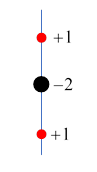
We begin with a dipole pointing along the $z$ axis, and displace it along the $z$ axis. Represent this by the charge distribution $Q_0$ at $\left(0,0,\frac{1}{2}\right)$ and $\left(0,0,-\frac{1}{2}\right)$ and $-2Q_0$ at the origin. This gives the quadrupole tensor

$Q_{\alpha \beta }=Q_0\left(\begin{array}{ccc}-\frac{1}{2}& 0& 0\\ 0& -\frac{1}{2}& 0\\ 0& 0& 1\end{array}\right)=Q_0\left(\begin{array}{ccc}-\frac{1}{2}& 0& 0\\ 0& -\frac{1}{2}& 0\\ 0& 0& -\frac{1}{2}\end{array}\right)+Q_0\left(\begin{array}{ccc}0& 0& 0\\ 0& 0& 0\\ 0& 0& 1\frac{1}{2}\end{array}\right).$ 

We split it this way because the first (identity) tensor won't contribute to the radiation distribution

$\frac{d{P}_{\text{el quad}}}{d\Omega }=\frac{c^2{Z}_0}{2{\left(24\right)}^2{\pi }^2}{k}^6{\left|\widehat{\overrightarrow{r}}\times \overrightarrow{Q}\left(\widehat{\overrightarrow{r}}\right)\right|}^2,$

we'll just get

$\begin{array}{c}\frac{d{P}_{\text{el quad}}}{d\Omega }=\frac{c^2{Z}_0}{2{\left(24\right)}^2{\pi }^2}{k}^6.{\left(1\frac{1}{2}\right)}^2{Q}_0^2{\left|\left(\begin{array}{ccc}\sin \theta & 0& \cos \theta \end{array}\right)\times \left(\begin{array}{ccc}0& 0& \cos \theta \end{array}\right)\right|}^2\\ =\frac{c^2{Z}_0{k}^6}{512{\pi }^2}{Q}_0^2{\sin }^2\theta {\cos }^2\theta .\end{array}$ 

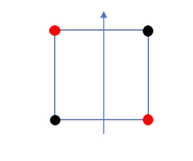
Another kind of quadrupole is the laterally displaced opposite dipole.  This would give different radiation patterns if rotated about the axis shown, or about an axis through the center of the square perpendicular to the plane.

These are left as an exercise for the reader.

previous  index  next