59  Scattering of EM Waves

    Michael Fowler, UVa

(Jackson chapter 10)

Introduction

We'll begin by considering scattering at long wavelengths, by which we mean wavelengths $\lambda \gg d,$ the size of the object scattering the wave.  This means that to a good approximation, at any instant of time we can regard the scatterer as being in a constant electric field (with the time dependence $e^{-i\omega t},$ of course). 

Thus we begin by finding the response of the scatterer to a constant field (and we need to check that the material can respond sufficiently quickly to follow the changing field).  For a spherical scatterer, the simplest system, we only need to find the dipole response.  Higher order terms only come into play if the wavelength becomes comparable to the size of the system.

We take an ingoing plane wave,

${\overrightarrow{E}}_{\text{in}}={\overrightarrow{\epsilon }}_0{E}_0{e}^{ik{\widehat{\overrightarrow{n}}}_0\cdot \overrightarrow{r}},{\overrightarrow{H}}_{\text{in}}={\widehat{\overrightarrow{n}}}_0\times {\overrightarrow{E}}_{\text{in}}/Z_0.$ 

 In general, such a field will induce an electric dipole moment $\overrightarrow{p}$ and magnetic dipole moment $\overrightarrow{m}$ in the small scatterer, and far away the scattered radiation will have leading terms (as derived in the previous lecture)

$\begin{array}{l}{\overrightarrow{E}}_{\text{sc}}=\frac{1}{4\pi {\epsilon }_0}{k}^2\frac{e^{ikr}}{r}\left[\left(\widehat{\overrightarrow{r}}\times \overrightarrow{p}\right)\times \widehat{\overrightarrow{r}}-\widehat{\overrightarrow{r}}\times \overrightarrow{m}/c\right],\\ {\overrightarrow{H}}_{\text{sc}}=\widehat{\overrightarrow{r}}\times {\overrightarrow{E}}_{\text{sc}}/Z_0.\end{array}$ 

The scattering differential cross-section is defined as follows: for unit ingoing flux (watts/m^-2) with polarization ${\overrightarrow{\epsilon }}_0,$ what is the outgoing$—$scattered$—$power/solid angle having polarization $\overrightarrow{\epsilon }$?  (Of course, the outgoing polarization is polarized in the direction ${\overrightarrow{E}}_{\text{sc}},$ but this has component ${\overrightarrow{\epsilon }}^{\ast }\cdot {\overrightarrow{E}}_{\text{sc}}$ in the direction $\overrightarrow{\epsilon }.$ The complex conjugation is introduced to take care of circularly polarized light, it doesn't matter for ordinary linearly polarized light.)  Writing this as an equation, quoting Jackson but simplifying,

$\frac{d\sigma }{d\Omega }\left(\widehat{\overrightarrow{r}},\overrightarrow{\epsilon };{\widehat{\overrightarrow{n}}}_0,{\overrightarrow{\epsilon }}_0\right)=\frac{r^2\frac{1}{2Z_0}{\left|{\overrightarrow{\epsilon }}^{\ast }\cdot {\overrightarrow{E}}_{\text{sc}}\right|}^2}{\frac{1}{2Z_0}{\left|{\overrightarrow{\epsilon }}_0{}^{\ast }\cdot {\overrightarrow{E}}_{\text{in}}\right|}^2}.$ 

So if we only have dipole scattering:

$\frac{d\sigma }{d\Omega }\left(\widehat{\overrightarrow{r}},\overrightarrow{\epsilon };{\widehat{\overrightarrow{n}}}_0,{\overrightarrow{\epsilon }}_0\right)=\frac{1}{E_0^2}{\left(\frac{1}{4\pi {\epsilon }_0}\right)}^2{k}^4{\left|{\overrightarrow{\epsilon }}^{\ast }\cdot \overrightarrow{p}+\left(\widehat{\overrightarrow{r}}\times {\overrightarrow{\epsilon }}^{\ast }\right)\cdot \overrightarrow{m}/c\right|}^2.$ 

Here $E_0^2$ is the incident power flow density.  Note that the scattering goes as $k^4,$ Rayleigh's law, of course $\omega =ck.$ 

Scattering from a Small Dielectric Sphere

"Small" here means having diameter much less than the wavelength of the scattered light, $a\ll \lambda .$ For such an object, the incoming wave is effectively a spatially constant, but time-oscillating, electric field, and assuming the sphere's electric response is much faster than the wave oscillation time, we can use the electrostatic result derived long ago, that the incoming field will induce a dipole.  For a sphere with dielectric constant ${\epsilon }_1,$ that earlier result is

$\overrightarrow{p}=4\pi {\epsilon }_0{a}^3{\overrightarrow{E}}_{\text{in}}\left(\frac{{\epsilon }_r-1}{{\epsilon }_r+2}\right),{\epsilon }_r=\frac{{\epsilon }_1}{{\epsilon }_0}.$ 

Putting this into the differential scattering cross section formula we just found,

$\begin{array}{c}\frac{d\sigma }{d\Omega }\left(\widehat{\overrightarrow{r}},\overrightarrow{\epsilon };{\widehat{\overrightarrow{n}}}_0,{\overrightarrow{\epsilon }}_0\right)=\frac{1}{E_0^2}{\left(\frac{1}{4\pi {\epsilon }_0}\right)}^2{k}^4{\left|{\overrightarrow{\epsilon }}^{\ast }\cdot \overrightarrow{p}\right|}^2\\ =k^4{a}^6{\left|\frac{{\epsilon }_r-1}{{\epsilon }_r+2}\right|}^2{\left|{\overrightarrow{\epsilon }}^{\ast }\cdot {\overrightarrow{\epsilon }}_0\right|}^2\end{array}$ 

since the induced dipole is in the direction of the incoming electric field.

But more relevant to, say, the blue sky, is scattering of unpolarized incoming light: all polarization directions perpendicular to the incoming direction of propagation are equally likely, so we must take an average. Of course, we'll still get a result depending on the measured outgoing polarization, as will become evident. 

To perform the averaging over incoming polarization directions, Jackson draws a rather unclear (in my opinion) diagram, which we'll explain:

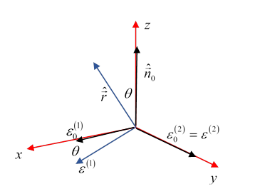
Begin with a set of Cartesian axes, and orient the incoming wave direction ${\widehat{\overrightarrow{n}}}_0$ along the $z$ axis. For chosen outgoing direction (in which the outgoing polarization will be measured) $\widehat{\overrightarrow{r}}$ (Jackson's $\widehat{\overrightarrow{n}}$ ) we take ${\widehat{\overrightarrow{n}}}_0,\widehat{\overrightarrow{r}}$ to define the $x,z$ plane, and the scattering angle is $\theta .$ 

Jackson calls the ingoing polarization basis vectors ${\overrightarrow{\epsilon }}_0^{\left(1\right)},{\overrightarrow{\epsilon }}_0^{\left(2\right)}$, along the $x,y$ axes. The outgoing polarization basis states are given by rotating these basis vectors about the $y$ axis (see diagram) to give a new ${\overrightarrow{\epsilon }}^{\left(1\right)},$ (in the $x,z$ plane),  but ${\epsilon }^{\left(2\right)}={\overrightarrow{\epsilon }}_0^{\left(2\right)}$ (see figure).

Now, leaving the outgoing polarization direction ${\overrightarrow{\epsilon }}^{\left(1\right)}$ constant, we'll average over all possible ingoing polarizations,  ${\overrightarrow{\epsilon }}_0$ 's, their tips lie on the unit circle in the $x,y$ plane.  Since we're evaluating the average value of ${\left|{\overrightarrow{\epsilon }}^{\left(1\right)}\cdot {\overrightarrow{\epsilon }}_0\right|}^2,$  the only relevant component of the incoming polarization is its $x$ component, having magnitude $\cos \varphi ,$ say.  This is to be multiplied by the $\cos \theta$ from the dot product, the square ${\left|{\overrightarrow{\epsilon }}^{\ast }\cdot {\overrightarrow{\epsilon }}_0\right|}^2$ averaging to $\frac{1}{2}{\cos }^2\theta ,$ the $\frac{1}{2}$ being $\overline{{\cos }^2\varphi },$ so for polarization like this parallel to the scattering plane (defined by ingoing and outgoing wave vectors)

$\frac{d{\sigma }_{\parallel }}{d\Omega }==k^4{a}^6{\left|\frac{{\epsilon }_r-1}{{\epsilon }_r+2}\right|}^2{\cos }^2\theta .$ 

For polarization perpendicular to the plane of scattering, the outgoing polarization vector is in the same plane as the ingoing polarization vector, so the analysis is even simpler: the ${\cos }^2\theta$ term is not there:

$\frac{d{\sigma }_{\perp }}{d\Omega }=k^4{a}^6{\left|\frac{{\epsilon }_r-1}{{\epsilon }_r+2}\right|}^2.$ 

The polarization of the scattered radiation is defined by

$\Pi \left(\theta \right)=\frac{\frac{d{\sigma }_{\perp }}{d\Omega }-\frac{d{\sigma }_{\parallel }}{d\Omega }}{\frac{d{\sigma }_{\perp }}{d\Omega }+\frac{d{\sigma }_{\parallel }}{d\Omega }}.$ 

The dipole scattering from a small dielectric sphere has polarization

$\Pi \left(\theta \right)=\frac{{\sin }^2\theta }{1+{\cos }^2\theta }$ 

and differential cross section summed over scattered polarization

$\frac{d\sigma }{d\Omega }=k^4{a}^6{\left|\frac{{\epsilon }_r-1}{{\epsilon }_r+2}\right|}^2\frac{1}{2}\left(1+{\cos }^2\theta \right),$ 

for a total cross section

$\sigma =\frac{8\pi }{3}{k}^4{a}^6{\left|\frac{{\epsilon }_r-1}{{\epsilon }_r+2}\right|}^2.$ 

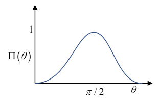
The polarization $\Pi \left(\theta \right)$ is maximal, equal to unity, at $\theta =\pi /2,$ and falls away symmetrically to zero at $\theta =0,\pi .$ Near $\theta =0,$ it goes as ${\theta }^2/2.$ (Note that Jackson (p 459) plots the polarization as a function of $\cos \theta ,$ not $\theta .$ )

How does this affect the blue sky?  Look at different parts of the sky on a clear day, using a polaroid filter, or polarized sunglasses. The very polarized light is that from the Sun but scattered through 90 degrees. Figure out where to look, then check the plane of polarization for that light.

Scattering by a Small Perfectly Conducting Sphere

The electric field induces an electric dipole, the spatially constant electric field ( $\lambda \gg a$ ) has potential $-E_{\text{inc}}r\cos \theta ,$ inside the sphere, of course, $\overrightarrow{E}\equiv 0,$ the induced dipole has potential $\frac{1}{4\pi {\epsilon }_0}\frac{p}{r^2}\cos \theta ,$ the tangential component of the electric field must be zero at $r=a,$ from which

$\overrightarrow{p}=4\pi {\epsilon }_0{a}^3{\overrightarrow{E}}_{\text{inc}}.$ 

But there's also the magnetic field, inducing a magnetic dipole, we can use the scalar potential, the field has potential $-{\mu }_0{H}_{0}r\cos \theta ,$ the induced dipole potential is $\frac{{\mu }_0}{4\pi }\frac{m}{r^2}\cos \theta$ but now the normal component of the total field is zero, so $-{\mu }_0{H}_0-\frac{2{\mu }_0}{4\pi }\frac{m}{a^3}=0,$  so

$\overrightarrow{m}=-2\pi a^3{\overrightarrow{H}}_{\text{inc}}.$ 

So, the incoming $\overrightarrow{E}$ and $\overrightarrow{H}$ fields induce perpendicular electric and magnetic dipoles!  We must therefore use the full formula

$\frac{d\sigma }{d\Omega }\left(\widehat{\overrightarrow{r}},\overrightarrow{\epsilon };{\widehat{\overrightarrow{n}}}_0,{\overrightarrow{\epsilon }}_0\right)=\frac{1}{E_0^2}{\left(\frac{1}{4\pi {\epsilon }_0}\right)}^2{k}^4{\left|{\overrightarrow{\epsilon }}^{\ast }\cdot \overrightarrow{p}+\left(\widehat{\overrightarrow{r}}\times {\overrightarrow{\epsilon }}^{\ast }\right)\cdot \overrightarrow{m}/c\right|}^2.$ 

Exercise: Draw a sketch of the vector directions $\overrightarrow{\epsilon }\equiv {\overrightarrow{E}}_{\text{inc}},{\overrightarrow{H}}_{\text{inc}},\overrightarrow{p},\overrightarrow{m},\widehat{\overrightarrow{r}}$ and explain why there is strong backward scattering, as a result of interference between the electric and magnetic terms. What about forward scattering?

For details of the polarization of the scattered radiation, see Jackson (or work it out).

Collections of Scatterers

Jackson 10.1 D

Suppose we have a number of identical small scatterers, distributed in space at random points ${\overrightarrow{r}}_1,{\overrightarrow{r}}_2,\dots ,{\overrightarrow{r}}_N$.  Take light coming in in direction ${\widehat{\overrightarrow{n}}}_0$ scattered to outward direction $\widehat{\overrightarrow{r}}.$ 

The incoming wave at ${\overrightarrow{r}}_j,$ the position of the j ^th  scatterer, includes a phase factor $e^{ik{\widehat{\overrightarrow{n}}}_0\cdot {\overrightarrow{r}}_j}$. Similarly, the outgoing scattered wave will have a factor $e^{-ik\widehat{\overrightarrow{r}}\cdot {\overrightarrow{r}}_j}$, so overall the outgoing wave will have a factor $e^{i\overrightarrow{q}\cdot {\overrightarrow{r}}_j},$ $\overrightarrow{q}=k\left({\widehat{\overrightarrow{n}}}_0-\widehat{\overrightarrow{r}}\right)$ compared with an identical scatterer located at the origin. Therefore, if we add the scattering from a distribution of scatterers, assuming they are dilute enough that we can ignore multiple scattering (meaning each independently just sees the incoming field, no effect from the others) the cross section is multiplied by the structure factor:   

$F\left(\overrightarrow{q}\right)={\left|{\displaystyle \sum _j{e}^{i\overrightarrow{q}\cdot {\overrightarrow{r}}_j}}\right|}^2=\left({\displaystyle \sum _j{e}^{-i\overrightarrow{q}\cdot {\overrightarrow{r}}_j}}\right)\left({\displaystyle \sum _k{e}^{i\overrightarrow{q}\cdot {\overrightarrow{r}}_k}}\right).$ 

If the $N$ scatterers are randomly placed,  all the $j=k$ terms in the product contribute 1, the others have random phases, and cancel on average. We conclude that the total scattering equals that for a single scatterer multiplied by the number of scatterers.

Perturbation Theory of Scattering: Blue Sky, etc.

General Theory

We begin with an ingoing monochromatic wave, in a medium having constant $\epsilon ,\mu .$  now suppose that in some finite region there are small fluctuations, say $\epsilon ={\epsilon }_0+\delta \epsilon \left(\overrightarrow{r}\right).$ Then we simply write out the exact Maxwell equations again, throw away terms of second-order in the small fluctuations, and derive the Helmholtz equations, which now have a right hand side from the fluctuation, to leading order

$\left({\nabla }^2+k^2\right)\overrightarrow{D}=-\overrightarrow{\nabla }\times \overrightarrow{\nabla }\times \left(\delta \epsilon \left(\overrightarrow{r}\right)/{\epsilon }_0\right)\overrightarrow{D}.$ 

We now see that the local change in dielectric constant acts as a new source term for the electric field, and similar but magnetic terms will appear for fluctuations $\delta \mu \left(\overrightarrow{r}\right).$ 

So we first solve the constant ${\epsilon }_0$ case (or we're given it as the ingoing wave) then we substitute that on the right-hand side to find the generated scattered wave, the left-hand side.

It's obviously an approximation to put the unperturbed wave on the right, and can be refined by putting the newly solved wave, plus scattering, there.  Repeating this process is called "perturbation theory". The first correction alone, with the unperturbed field on the right, was first used by Lord Rayleigh.  It was reinvented when quantum mechanics came along, and is now called the Born approximation.

Jackson applies this to the dielectric sphere: it gives the previously found result in the low frequency limit, and for forward scattering at all frequencies.

Exercise: Check that you can find Jackson's result for his integral in (10.31). This integral appears in other places in physics.

Now for the blue sky. Assume that individual molecules, located at ${\overrightarrow{r}}_j,$ have dipole moments ${\overrightarrow{p}}_j={\epsilon }_0{\gamma }_{\text{mol}}\overrightarrow{E}\left({\overrightarrow{r}}_j\right),$ then the differential cross section, adapting our previous result for dipole moment induced in a sphere by an electric field, is

$\frac{d\sigma }{d\Omega }=\frac{k^4}{16{\pi }^2}{\left|{\gamma }_{\text{mol}}\right|}^2{\left|{\overrightarrow{\epsilon }}^{\ast }\cdot {\overrightarrow{\epsilon }}_0\right|}^{2}F\left(\overrightarrow{q}\right)$ 

and for $N$ scatterers, $F\left(\overrightarrow{q}\right)$ is just $N.$ For a dilute gas,  the dielectric constant is ${\epsilon }_r\cong 1+N{\gamma }_{\text{mol}},$ $N$ now being the number density.  The scattering cross section per molecule of gas is then

$\sigma \simeq \frac{k^4}{6\pi N^2}{\left|{\epsilon }_r-1\right|}^2.$ 

This means that a plane wave with unit area cross section, on progressing by $dx,$ will encounter area $N\sigma dx$ of blockage, so the power in the wave will change by $dP=-PN\sigma dx,$ an attenuation coefficient $\alpha =N\sigma ,$ 

$P=P_0{e}^{-\alpha x}=P_0{e}^{-N\sigma x},\alpha =\frac{k^4}{6\pi N}{\left|{\epsilon }_r-1\right|}^2.$

For the atmosphere, ${\epsilon }_r-1=0.00059$ at sea level, but of course it decreases, and we're just talking ballpark here.   The number density $N\simeq 2.5\times {10}^{25},$ so the extinction length ${\alpha }^{-1}\sim {10}^{33}/k^4.$ The wavenumber of red light is about 10⁷ rads/m, giving an extinction length of order 100km.  The blue light would have a much shorter length, down by a factor of 6 or so.  These figures are only indications, the atmosphere thins out on this length scale, but we see we're in the right ballpark—the Sun does look very red at sunset, and the scattered light is certainly predominantly blue.

Density Fluctuations, Critical Opalescence

Light is scattered by variations in the dielectric constant.  For gases or liquids, this is usually proportional to density. Therefore, variations in density will scatter light. The amplitude of density variations driven by thermal fluctuations depends on the compressibility: if a gas changes volume substantially under small pressure changes, there will be large variations.

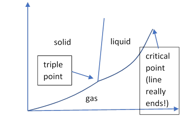
This is most dramatically manifested at the critical point: the liquid-gas interface between the triple point and the critical point is a first order phase transition, with finite density change. A fluid at a point on that curve (with gravity) will divide, with liquid in the lower half of the container. (Without gravity, the liquid will be in drops or bigger.) At the critical point, the fluids become identical, and above that point a container will fill uniformly with the fluid.  But right at the critical point, although the two densities become identical, the compressibility diverges—so small thermal fluctuations drive huge density fluctuations, hence big dielectric constant fluctuations, and a lot of light scattering: the fluid becomes opaque.

previous  index  next