previous  home  next  PDF

2. The Calculus of Variations

Michael Fowler

Introduction

We’ve seen how Whewell solved the problem of the equilibrium shape of chain hanging between two places, by finding how the forces on a length of chain, the tension at the two ends and its weight, balanced. We’re now going to look at a completely different approach: the equilibrium configuration is an energy minimum, so small deviations from it can only make second-order changes in the gravitational potential energy. Here we’ll find how analyzing that leads to a differential equation for the curve, and how the technique developed can be successfully applied of a vast array of problems. 

The Catenary and the Soap Film

The catenary is the curved configuration $y=y\left(x\right)$ of a uniform inextensible rope with two fixed endpoints at rest in a constant gravitational field.  That is to say, it is the curve that minimizes the gravitational potential energy

$$J\left[y\left(x\right)\right]=2\pi {\displaystyle \underset{x_1}{\overset{x_2}{\int }}yds}=2\pi {\displaystyle \underset{x_1}{\overset{x_2}{\int }}y\sqrt{1+{y^{\prime }}^2}dx},\left(y^{\prime }=dy/dx\right)$$ where we have taken the rope density and gravity both equal to unity for mathematical convenience.  Usually in calculus we minimize a function with respect to a single variable, or several variables. Here the potential energy is a function of a function, equivalent to an infinite number of variables, and our problem is to minimize it with respect to arbitrary small variations of that function.  In other words, if we nudge the chain somewhere, and its motion is damped by air or internal friction, it will settle down again in the catenary configuration. 

Formally speaking, there will be no change in that potential energy to leading order if we make an infinitesimal change in the curve, $y\left(x\right)\to y\left(x\right)+\delta y\left(x\right)$ (subject of course to keeping the length the same, that is $\delta {\displaystyle \int ds}=0$.) 

This method of solving the problem is called the calculus of variations: in ordinary calculus, we make an infinitesimal change in a variable, and compute the corresponding change in a function, and if it’s zero to leading order in the small change, we’re at an extreme value.

(Nitpicking footnote:  Actually this assumes the second order term is nonzero—what about $x^3$ near the origin? But such situations are infrequent in the problems we’re likely to encounter.)

The difference here is that the potential energy of the hanging change isn’t just a function of a variable, or even of a number of variables—it’s a function of a function, it depends on the position of every point on the chain (in the limit of infinitely small links, that is, or equivalently a continuous rope).

So, we’re looking for the configuration where the potential energy doesn’t change to first order for any infinitesimal change in the curve of its position, subject to fixed endpoints, and a fixed chain length.

As a warm up, we’ll consider a simpler—but closely related—problem.

A Soap Film Between Two Horizontal Rings: the Euler-Lagrange Equation

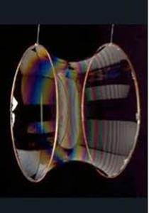This problem is very similar to the catenary:  surface tension will pull the soap film to the minimum possible total area compatible with the fixed boundaries (and neglecting gravity, which is a small effect).

(Interestingly, this problem is also closely related to string theory:  as a closed string propagates, its path traces out as “world sheet” and the string dynamics is determined by that sheet having minimal area.)

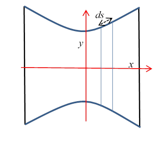Taking the axis of rotational symmetry to be the $x$ -axis, and the radius $y\left(x\right)$, we need to find the function $y\left(x\right)$ that minimizes the total area ( $ds$ is measured along the curve of the surface).  Think of the soap film as a sequence of rings or collars, of radius $y,$ and therefore area $2\pi yds.$ The total area is given by integrating, adding all these incremental collars,

$J\left[y\left(x\right)\right]=2\pi {\displaystyle \underset{x_1}{\overset{x_2}{\int }}yds}=2\pi {\displaystyle \underset{x_1}{\overset{x_2}{\int }}y\sqrt{1+{y^{\prime }}^2}dx}$

subject to given values of $y$ at the two ends. (You might be thinking at this point: isn’t this identical to the catenary equation?  The answer is yes, but the chain has an additional requirement: it has a fixed length.  The soap film is not constrained in that way, it can stretch or contract to minimize the total area, so this is a different problem!)

That is, we want $\delta J=0$ to first order, if we make a change $y\left(x\right)\to y\left(x\right)+\delta y\left(x\right)$. Of course, this also means $y^{\prime }\left(x\right)\to y^{\prime }\left(x\right)+\delta y^{\prime }\left(x\right)$ where $\delta y^{\prime }=\delta \left(dy/dx\right)=\left(d/dx\right)\delta y$.

General Method for the Minimization Problem

To emphasize the generality of the method, we’ll just write

$J\left[y\right]={\displaystyle \underset{x_1}{\overset{x_2}{\int }}f\left(y,y^{\prime }\right)dx}\left(y^{\prime }=dy/dx\right)$.

Then under any infinitesimal variation $\delta y\left(x\right)$ (equal to zero at the fixed endpoints)

$$\delta J\left[y\right]={\displaystyle \underset{x_1}{\overset{x_2}{\int }}\left[\frac{\partial f\left(y,y^{\prime }\right)}{\partial y}\delta y\left(x\right)+\frac{\partial f\left(y,y^{\prime }\right)}{\partial y^{\prime }}\delta y^{\prime }\left(x\right)\right]dx}=0.$$

To make further progress, we write $\delta y^{\prime }=\delta \left(dy/dx\right)=\left(d/dx\right)\delta y$, then integrate the second term by parts, remembering $\delta y=0$ at the endpoints, to get

$$\delta J\left[y\right]={\displaystyle \underset{x_1}{\overset{x_2}{\int }}\left[\frac{\partial f\left(y,y^{\prime }\right)}{\partial y}-\frac{d}{dx}\left(\frac{\partial f\left(y,y^{\prime }\right)}{\partial y^{\prime }}\right)\right]\delta y\left(x\right)dx}=0.$$

Since this is true for any infinitesimal variation, we can choose a variation which is only nonzero near  one point in the interval, and deduce that

$$\frac{\partial f\left(y,y^{\prime }\right)}{\partial y}-\frac{d}{dx}\left(\frac{\partial f\left(y,y^{\prime }\right)}{\partial y^{\prime }}\right)=0.$$

This general result is called the Euler-Lagrange equation.  It’s very important$—$you’ll be seeing it again.

An Important First Integral of the Euler-Lagrange Equation

It turns out that, since the function $f$ does not contain $x$ explicitly, there is a simple first integral of this equation.  Multiplying throughout by $y^{\prime }=dy/dx$,

$$\frac{\partial f\left(y,y^{\prime }\right)}{\partial y}\frac{dy}{dx}-\frac{d}{dx}\left(\frac{\partial f\left(y,y^{\prime }\right)}{\partial y^{\prime }}\right)y^{\prime }=0.$$

Since $f$ doesn’t depend explicitly on $x$, we have

$$\frac{df}{dx}=\frac{\partial f}{\partial y}\frac{dy}{dx}+\frac{\partial f}{\partial y^{\prime }}\frac{d{y}^{\prime }}{dx}$$

 and using this to replace $\frac{\partial f\left(y,y^{\prime }\right)}{\partial y}\frac{dy}{dx}$ in the preceding equation gives

$$\frac{df}{dx}-\frac{\partial f}{\partial y^{\prime }}\frac{d{y}^{\prime }}{dx}-\frac{d}{dx}\left(\frac{\partial f\left(y,y^{\prime }\right)}{\partial y^{\prime }}\right)y^{\prime }=0,$$

then multiplying by − (to match the equation as usually written) we have

$$\frac{d}{dx}\left(y^{\prime }\frac{\partial f}{\partial y^{\prime }}-f\right)=0,$$

giving a first integral

$$y^{\prime }\frac{\partial f}{\partial y^{\prime }}-f=\text{constant}\text{.}$$

For the soap film between two rings problem,

$$f\left(y,y^{\prime }\right)=y\sqrt{1+{y^{\prime }}^2},$$

so the Euler-Lagrange equation is

$$\sqrt{1+{y^{\prime }}^2}-\frac{d}{dx}\frac{y{y}^{\prime }}{\sqrt{1+{y^{\prime }}^2}}=0.$$

and has first integral

$$y^{\prime }\frac{\partial f}{\partial y^{\prime }}-f=\frac{y{y^{\prime }}^2}{\sqrt{1+{y^{\prime }}^2}}-y\sqrt{1+{y^{\prime }}^2}=-\frac{y}{\sqrt{1+{y^{\prime }}^2}}=\text{constant}\text{.}$$

We’ll write

$$\frac{y}{\sqrt{1+{y^{\prime }}^2}}=a,$$

with a the constant of integration, which will depend on the endpoints.

This is a first-order differential equation, and can be solved. 

Rearranging,

$$\frac{dy}{dx}=\sqrt{{\left(\frac{y}{a}\right)}^2-1},$$

or

$$dx=\frac{ady}{\sqrt{y^2-a^2}}.$$

The standard substitution here is $y=a\cosh \xi$, from which

$$y=a\cosh \left(\frac{x-b}{a}\right).$$

Here $b$ is the second constant of integration, the fixed endpoints determine $a,b$.                          $$

The Soap Film and the Chain

We see that the soap film profile function and the hanging chain have identical analytic form.  This is not too surprising, because the potential energy of the hanging chain in simplified units is just

$${\displaystyle \int y}ds={\displaystyle \int y}{\left(1+{y^{\prime }}^2\right)}^{\frac{1}{2}}dx,$$

the same as the area function for the soap film.  But there’s an important physical difference: the chain has a fixed length.  The soap film is free to adjust its “length” to minimize the total area. The chain isn’t—it’s constrained.  How do we deal with that? 

Lagrange Multipliers

The problem of finding minima (or maxima) of a function subject to constraints was first solved by Lagrange.  A simple example will suffice to show the method.

Imagine we have some smooth curve in the $\left(x,y\right)$ plane that does not pass through the origin, and we want to find the point on the curve that is its closest approach to the origin.  A standard illustration is to picture a winding road through a bowl shaped valley, and ask for the low point on the road.  (We’ll also assume that $x$ determines $y$ uniquely, the road doesn’t double back, etc.  If it does, the method below would give a series of locally closest points to the origin, we would need to go through them one by one to find the globally closest point.)

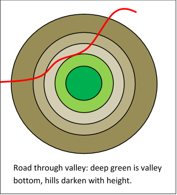Let’s write the curve, the road, $g\left(x,y\right)=0$ (the wiggly red line in the figure below).

To find the closest approach point algebraically, we need to minimize $f\left(x,y\right)=x^2+y^2$ (square of distance to origin) subject to the constraint $g\left(x,y\right)=0$.

In the figure, we’ve drawn curves

$f\left(x,y\right)=x^2+y^2=a^2$ 

for a range of values of $a$ (the circles centered at the origin).

We need to find the point of intersection of $g\left(x,y\right)=0$ with the smallest circle it intersects$—$and it’s clear from the figure that it must touch that circle (if it crosses, it will necessarily get closer to the origin).

Therefore, at that point, the curves $g\left(x,y\right)=0$ and $f\left(x,y\right)=a_{\min }^2$ are parallel.

Therefore the normals to the curves are also parallel:

$\left(\partial f/\partial x,\partial f/\partial y\right)=\lambda \left(\partial g/\partial x,\partial g/\partial y\right)$. 

(Note:  yes, those are the directions of the normals— for an infinitesimal displacement along the curve $f\left(x,y\right)$ =constant, $0=df=\left(\partial f/\partial x\right)dx+\left(\partial f/\partial y\right)dy$, so the vector $\left(\partial f/\partial x,\partial f/\partial y\right)$ is perpendicular to $\left(dx,dy\right)$. This is also analogous to the electric field $\overrightarrow{E}=-\overrightarrow{\nabla }\phi$ being perpendicular to the equipotential $\phi \left(x,y\right)=\text{constant}\text{.}$ )  

The constant $\lambda$ introduced here is called a Lagrange multiplier.  It’s just the ratio of the lengths of the two normal vectors (of course, “normal” here means the vectors are perpendicular to the curves, they are not normalized to unit length!)  We can find $\lambda$ in terms of $x,y$ but at this point we don’t know their values.

The equations determining the closest approach to the origin can now be written:

$$\begin{array}{l}\frac{\partial }{\partial x}\left(f-\lambda g\right)=0,\\ \frac{\partial }{\partial y}\left(f-\lambda g\right)=0,\\ \frac{\partial }{\partial \lambda }\left(f-\lambda g\right)=0.\end{array}$$

(The third equation is just $g\left(x_{\min },y_{\min }\right)=0$, meaning we’re on the road.)

We have transformed a constrained minimization problem in two dimensions to an unconstrained minimization problem in three dimensions!

The first two equations can be solved to find λ  and the ratio $x/y$, the third equation then gives $x,y$ separately. 

Exercise for the reader:   Work through this for $g\left(x,y\right)=x^2-2xy-y^2-1.$ (There are two solutions because the curve $g=0$ is a hyperbola with two branches.)

Lagrange multipliers are widely used in economics, and other useful subjects such as traffic optimization.

Lagrange Multiplier for the Chain

The catenary is generated by minimizing the potential energy of the hanging chain given above,

$$J\left[y\left(x\right)\right]={\displaystyle \int y}ds={\displaystyle \int y}{\left(1+{y^{\prime }}^2\right)}^{\frac{1}{2}}dx,$$

but now subject to the constraint of fixed chain length, $L\left[y\left(x\right)\right]={\displaystyle \int ds=\ell .}$

The Lagrange multiplier method generalizes in a straightforward way from variables to variable functions.  In the curve example above, we minimized $f\left(x,y\right)=x^2+y^2$ subject to the constraint $g\left(x,y\right)=0.$  What we need to do now is minimize $J\left[y\left(x\right)\right]$ subject to the constraint $L\left[y\left(x\right)\right]-\ell =0.$ 

For the minimum curve $y\left(x\right)$ and the correct (so far unknown) value of $\lambda$, an arbitrary infinitesimal variation of the curve will give zero first-order change in $J-\lambda L$, we write this as  

$$\delta \left\{J\left[y\left(x\right)\right]-\lambda L\left[y\left(x\right)\right]\right\}=\delta \left\{{\displaystyle \underset{x_1}{\overset{x_2}{\int }}\left(y-\lambda \right)ds}\right\}=\delta \left\{{\displaystyle \underset{x_1}{\overset{x_2}{\int }}\left(y-\lambda \right)\sqrt{1+{y^{\prime }}^2}dx}\right\}=0.$$ Remarkably, the effect of the constraint is to give a simple adjustable parameter, the origin in the $y$ direction, so that we can satisfy the endpoint and length requirements.

The solution to the equation follows exactly the route followed for the soap film, leading to the first integral

$$\frac{y-\lambda }{{\left(1+{y^{\prime }}^2\right)}^{\frac{1}{2}}}=a,$$

with $a$ a constant of integration, which will depend on the endpoints.

Rearranging,

$$\frac{dy}{dx}=\sqrt{{\left(\frac{y-\lambda }{a}\right)}^2-1},$$

or

$$dx=\frac{ady}{\sqrt{{\left(y-\lambda \right)}^2-a^2}}.$$

The standard substitution here is $y-\lambda =c\cosh \xi$, we find

$$y=\lambda +a\cosh \left(\frac{x-b}{a}\right).$$

Here $b$ is the second constant of integration, the fixed endpoints and length give $\lambda ,a,b.$  In general, the equations must be solved numerically. To get some feel for why this will always work, note that changing $a$ varies how rapidly the cosh curve climbs from its low point of $\left(x,y\right)=\left(b,\lambda +a\right)$, increasing $a$ “fattens” the curve, then by varying $b,\lambda$ we can move that lowest point to the lowest point of the chain (or rather of the catenary, since it might be outside the range covered by the physical chain).

Algebraically, we know the curve can be written as $y=a\cosh \left(x/a\right)$, although at this stage we don’t know the constant $a$ or where the origin is. What we do know is the length of the chain, and the horizontal and vertical distances $\left(x_2-x_1\right)$ and $\left(y_2-y_1\right)$ between the fixed endpoints.   It’s straightforward to calculate that the length of the chain is $\ell =a\sinh \left(x_2/a\right)-a\sinh \left(x_1/a\right)$ , and the vertical distance $v$ between the endpoints is $v=a\cosh \left(x_2/a\right)-a\cosh \left(x_1/a\right)$ from which ${\ell }^2-v^2=4a^2{\sinh }^2\left[\left(x_2-x_1\right)/2a\right]$.   All terms in this equation are known except $a$, which can therefore be found numerically.   (This is in Wikipedia, among other places.)

Exercise:  try applying this reasoning to finding $a$ for the soap film minimization problem.  In that case, we know $\left(x_1,y_1\right)$ and $\left(x_2,y_2\right)$, there is no length conservation requirement, to find $a$ we must eliminate the unknown $b$ from the equations $y_1=a\cosh \left(\left(x_1-b\right)/a\right),$ $y_2=a\cosh \left(\left(x_2-b\right)/a\right).$ This is not difficult, but, in contrast to the chain, does not give $a$ in terms of $y_1-y_2$, instead, $y_1,y_2$ appear separately.  Explain, in terms of the physics of the two systems, why this is so different from the chain.

The Brachistochrone

Suppose you have two points, A and B, B is below A, but not directly below. You have some smooth, let’s say frictionless, wire, and a bead that slides on the wire.  The problem is to curve the wire from A down to B in such a way that the bead makes the trip as quickly as possible.

This optimal curve is called the “brachistochrone”, which is just the Greek for “shortest time”.

But what, exactly, is this curve, that is, what is $y\left(x\right)$, in the obvious notation?

This was the challenge problem posed by Johann Bernoulli to the mathematicians of Europe in a Journal run by Leibniz in June 1696. Isaac Newton was working fulltime running the Royal Mint, recoining England, and hanging counterfeiters.  Nevertheless, ending a full day’s work at 4 pm, and finding the problem delivered to him, he solved it by 4am the next morning, and sent the solution anonymously to Bernoulli. Bernoulli remarked of the anonymous solution “I recognize the lion by his clawmark”.

This was the beginning of the Calculus of Variations.

Here’s how to solve the problem:  we’ll take the starting point A to be the origin, and for convenience measure the $y$ -axis positive downwards.   This means the velocity at any point on the path is given by

$$\frac{1}{2}m{v}^2=mgy,v=\sqrt{2gy},$$

So measuring length along the path as $ds$ as usual, the time is given by

$$T={\displaystyle \underset{A}{\overset{B}{\int }}\frac{ds}{v}}={\displaystyle \underset{A}{\overset{B}{\int }}\frac{ds}{\sqrt{2gy}}}={\displaystyle \underset{0}{\overset{X}{\int }}\frac{\sqrt{1+{y^{\prime }}^2}dx}{\sqrt{2gy}}}.$$  Notice that this has the same form as the catenary equation, the only difference being that $y$ is replaced by $1/\sqrt{2gy}$, the integrand does not depend on $x,$ so we have the first integral:

$$y^{\prime }\frac{\partial f}{\partial y^{\prime }}-f=\text{constant,}f=\sqrt{\frac{1+{y^{\prime }}^2}{2gy}}.$$

That is,

$$\frac{{y^{\prime }}^2}{\sqrt{\left(1+{y^{\prime }}^2\right)2gy}}-\sqrt{\frac{1+{y^{\prime }}^2}{2gy}}=-\frac{1}{\sqrt{\left(1+{y^{\prime }}^2\right)2gy}}=\text{constant,}$$

so

$${\left(\frac{dy}{dx}\right)}^2+1=\frac{2a}{y}$$   $2a$ being a constant of integration (the 2 proves convenient).

Recalling that the curve starts at the origin A, it must begin by going vertically downward, since $y=0.$ For small enough $y$, we can approximate by ignoring the 1, so $\sqrt{2a}dx\cong \sqrt{y}dy$ , $\sqrt{2a}x\cong \raisebox{1ex}{$2$}\!\left/ \!\raisebox{-1ex}{$3$}\right.y^{3/2}$ .  The curve must however become horizontal if it gets as far down as $y=2a$, and it cannot go below that level.

Rearranging in order to integrate,

$$dx=\frac{dy}{\sqrt{\frac{2a}{y}-1}}=\sqrt{\frac{y}{2a-y}}dy.$$  This is not a very appealing integrand.  It looks a little nicer on writing $y=a-az$,

$$dx=-a\sqrt{\frac{1-z}{1+z}}dz.$$  Now what?  We’d prefer for the expression inside the square root to be a perfect square, of course.  You may remember from high school trig that $1+\cos \theta =2{\cos }^2\left(\theta /2\right),1-\cos \theta =2{\sin }^2\left(\theta /2\right)$ . This gives immediately that

$$\frac{1-\cos \theta }{1+\cos \theta }={\tan }^2\frac{\theta }{2},$$  so the substitution $z=\cos \theta$ is what we need. 

Then $dz=-\sin \theta d\theta =-2\sin \left(\theta /2\right)\cos \left(\theta /2\right)d\theta ,$

$$dx=-a\tan \frac{\theta }{2}dz=2a\tan \frac{\theta }{2}\sin \frac{\theta }{2}\cos \frac{\theta }{2}d\theta =2a{\sin }^2\frac{\theta }{2}d\theta =a\left(1-\cos \theta \right)d\theta .$$  This integrates to give

$$\begin{array}{l}x=a\left(\theta -\sin \theta \right)\\ y=a\left(1-\cos \theta \right),\end{array}$$ where we’ve fixed the constant of integration so that the curve goes through the origin (at $\theta =0$ ).

To see what this curve looks like, first ignore the $\theta$ term in $x$, leaving $x=-a\sin \theta ,y=-a\cos \theta .$ Evidently as $\theta$ increases from zero, the point $\left(x,y\right)$ goes anticlockwise around a circle of radius $a$ centered at $\left(0,-a\right)$, that is, touching the $x$ -axis at the origin. 

Now adding the $\theta$ back in, this circular motion move steadily to the right, in such a way that the initial direction of the path is vertically down.  (For very small $\theta ,$ $y\sim {\theta }^2\gg x\sim {\theta }^3$ ).

Visualizing the total motion as $\theta$ steadily increases, the center moves from its original position at $\left(0,-a\right)$ to the right at a speed $a\theta .$ Meanwhile, the point is moving round the circle anticlockwise at this same speed. Putting together the center’s linear velocity with the corresponding angular velocity, we see the motion $\left(x\left(\theta \right),y\left(\theta \right)\right)$ is the path of a point on the rim of a wheel rolling without sliding along a road (upside down in our case, of course).  This is a cycloid.

Fastest Curve for Given Horizontal Distance

Suppose we want to find the curve a bead slides down to minimize the time from the origin to some specified horizontal displacement X, but we don’t care what vertical drop that entails.

Recall how we derived the equation for the curve:

At the minimum, under any infinitesimal variation $\delta y\left(x\right)$,

$$\delta J\left[y\right]={\displaystyle \underset{x_1}{\overset{x_2}{\int }}\left[\frac{\partial f\left(y,y^{\prime }\right)}{\partial y}\delta y\left(x\right)+\frac{\partial f\left(y,y^{\prime }\right)}{\partial y^{\prime }}\delta y^{\prime }\left(x\right)\right]dx}=0.$$ Writing $\delta y^{\prime }=\delta \left(dy/dx\right)=\left(d/dx\right)\delta y$, and integrating the second term by parts,

$$\delta J\left[y\right]={\displaystyle \underset{x_1}{\overset{x_2}{\int }}\left[\frac{\partial f\left(y,y^{\prime }\right)}{\partial y}-\frac{d}{dx}\left(\frac{\partial f\left(y,y^{\prime }\right)}{\partial y^{\prime }}\right)\right]\delta y\left(x\right)dx}+{\left[\frac{\partial f\left(y,y^{\prime }\right)}{\partial y^{\prime }}\delta y\left(x\right)\right]}_0^X=0.$$ In the earlier treatment, both endpoints were fixed, $\delta y\left(0\right)=\delta y\left(X\right)=0,$ so we dropped that final term.

However, we are now trying to find the fastest time for a given horizontal distance, so the final vertical distance is an adjustable parameter: $\delta y\left(X\right)\ne 0$.

As before, since $\delta J\left[y\right]=0$ for arbitrary $\delta y,$ we can still choose a $\delta y\left(x\right)$ which is only nonzero near some point not at the end, so we must still have 

$$\frac{\partial f\left(y,y^{\prime }\right)}{\partial y}-\frac{d}{dx}\left(\frac{\partial f\left(y,y^{\prime }\right)}{\partial y^{\prime }}\right)=0.$$ However, we must also have $\frac{\partial f\left(y\left(X\right),y^{\prime }\left(X\right)\right)}{\partial y^{\prime }}\delta y\left(X\right)=0,$ to first order for arbitrary infinitesimal $\delta y\left(X\right),$ (imagine a variation $\delta y$ only nonzero near the endpoint), this can only be true if $\frac{\partial f\left(y,y^{\prime }\right)}{\partial y^{\prime }}=0$ at $x=X.$

For the brachistochrone, $$f=\sqrt{\frac{1+{y^{\prime }}^2}{2gy}},\frac{\partial f}{\partial y^{\prime }}=\frac{y^{\prime }}{\sqrt{2gy\left(1+{y^{\prime }}^2\right)}}$$ so $\frac{\partial f\left(y,y^{\prime }\right)}{\partial y^{\prime }}=0$ at $x=X$ means that $f^{\prime }=0$, the curve is horizontal at the end $x=X.$ 

So the curve that delivers the bead a given horizontal distance the fastest is the half-cycloid (inverted) flat at the end.  It’s easy to see this fixes the curve uniquely:  think of the curve as generated by a rolling wheel, one half-turn of the wheel takes the top point to the bottom in distance X.

Exercise: how low does it go?

The Perfect Pendulum

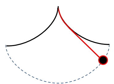Around the time of Newton, the best timekeepers were pendulum clocks$—$but the time of oscillation of a simple pendulum depends on its amplitude, although of course the correction is small for small amplitude.  The pendulum takes longer for larger amplitude.  This can be corrected for by having the string constrained between enclosing surfaces to steepen the pendulum’s path for larger amplitudes, and thereby speed it up. 

It turns out (and was proved geometrically by Newton) that the ideal pendulum path is a cycloid. Thinking in terms of the equivalent bead on a wire problem, with a symmetric cycloid replacing the circular arc of an ordinary pendulum, if the bead is let go from rest at any point on the wire, it will reach the center in the same time as from any other point.  So a clock with a pendulum constrained to such a path will keep very good time, and not be sensitive to the amplitude of swing. 

The proof involves similar integrals and tricks to those used above:

$$T\left(y_0\right)={\displaystyle \int \frac{ds}{\sqrt{2g\left(y-y_0\right)}}}={\displaystyle \int \frac{\sqrt{1+{y^{\prime }}^2}}{\sqrt{2g\left(y-y_0\right)}}dx}$$ and with the parameterization above, $y^{\prime }=\sin \theta /\left(1-\cos \theta \right)$, the integral becomes

$\sqrt{\frac{a}{g}}{\displaystyle \underset{{\theta }_0}{\overset{\pi }{\int }}\sqrt{\frac{1-\cos \theta }{\cos {\theta }_0-\cos \theta }}d\theta }$.

As before, we can now write $1-\cos \theta =2{\sin }^2\left(\theta /2\right)$, etc., to find that $T\left(y_0\right)$ is in fact independent of $y_0$. 

This is left as an exercise for the reader.  (Hint:  you may find ${\displaystyle {\int }_a^{b}dx/\sqrt{\left(x-a\right)\left(b-x\right)}}=\pi$ to be useful.  Can you prove this integral is correct?  Why doesn’t it depend on $a,b$?)

Exercise:  As you well know, a simple harmonic oscillator, a mass on a linear spring with restoring force $-kx$, has a period independent  of amplitude. Does this mean that a particle sliding on a cycloid is equivalent to a simple harmonic oscillator? Find out by expressing the motion as an equation $F=ma$ where the distance variable from the origin is s measured along the curve.

Check out cycloids here!

Calculus of Variations with Many Variables

We’ve found the equations defining the curve $y\left(x\right)$ along which the integral

$J\left[y\right]={\displaystyle \underset{x_1}{\overset{x_2}{\int }}f\left(y,y^{\prime }\right)dx}$

has a stationary value, and we’ve seen how it works in some two-dimensional curve examples. 

But most dynamical systems are parameterized by more than one variable, so we need to know how to go from a curve in $\left(x,y\right)$ to one in a space $\left(x,y_1,y_2,\dots y_n\right)$, and we need to minimize (say)

$$J\left[y_1,y_2,\dots y_n\right]={\displaystyle \underset{x_1}{\overset{x_2}{\int }}f\left(y_1,y_2,\dots y_n,y_1{}^{\prime },{y^{\prime }}_2,\dots {y^{\prime }}_n\right)dx}.$$ In fact, the generalization is straightforward: the path deviation simply becomes a vector,

$$\delta \overrightarrow{y}\left(x\right)=\left(\delta y_1\left(x\right),\delta y_2\left(x\right),\dots ,\delta y_n\left(x\right)\right)$$Then under any infinitesimal variation $\delta y\left(x\right)$ (writing also $y=\left(y_1,\dots y_n\right)$ )

$$\delta J\left[\overrightarrow{y}\right]={\displaystyle \underset{x_1}{\overset{x_2}{\int }}{\displaystyle \sum _{i=1}^n\left[\frac{\partial f\left(\overrightarrow{y},{\overrightarrow{y}}^{\prime }\right)}{\partial y_i}\delta y_i\left(x\right)+\frac{\partial f\left(\overrightarrow{y},{\overrightarrow{y}}^{\prime }\right)}{\partial {y^{\prime }}_i}\delta {y^{\prime }}_i\left(x\right)\right]}dx}=0.$$ Just as before, we take the variation zero at the endpoints, and integrate by parts to get now n separate equations for the stationary path:

$$\frac{\partial f\left(\overrightarrow{y},{\overrightarrow{y}}^{\prime }\right)}{\partial y_i}-\frac{d}{dx}\left(\frac{\partial f\left(\overrightarrow{y},{\overrightarrow{y}}^{\prime }\right)}{\partial {y^{\prime }}_i}\right)=0,i=1,\dots ,n.$$

Multivariable First Integral

Following and generalizing the one-variable derivation, multiplying the above equations one by one by the corresponding ${y^{\prime }}_i=d{y}_i/dx$ we have the n equations

$$\frac{\partial f\left(\overrightarrow{y},{\overrightarrow{y}}^{\prime }\right)}{\partial y_i}\frac{d{y}_i}{dx}-\frac{d}{dx}\left(\frac{\partial f\left(\overrightarrow{y},{\overrightarrow{y}}^{\prime }\right)}{\partial {y^{\prime }}_i}\right){y^{\prime }}_i=0.$$ Since $f$ doesn’t depend explicitly on $x$, we have

$\frac{df}{dx}={\displaystyle \sum _{i=1}^n\left(\frac{\partial f}{\partial y_i}\frac{d{y}_i}{dx}+\frac{\partial f}{\partial {y^{\prime }}_i}\frac{d{y^{\prime }}_i}{dx}\right)},$ 

and just as for the one-variable case, these equations give

$$\frac{d}{dx}\left({\displaystyle \sum _{i=1}^n{y^{\prime }}_i\frac{\partial f}{\partial {y^{\prime }}_i}}-f\right)=0,$$

and the (important!) first integral            ${\displaystyle \sum _{i=1}^n{y^{\prime }}_i\frac{\partial f}{\partial {y^{\prime }}_i}}-f=\text{constant}\text{.}$

previous  home  next  PDF