previous  home  next  PDF

17. Small Oscillations

Michael Fowler

Particle in a Well

We begin with the one-dimensional case of a particle oscillating about a local minimum of the potential energy $V\left(x\right).$  We’ll assume that near the minimum, call it $x_0$, the potential is well described by the leading second-order term, $V\left(x\right)=\frac{1}{2}{V}^{″}\left(x_0\right){\left(x-x_0\right)}^2$, so we’re taking the zero of potential at $x_0,$ assuming that the second derivative $V^{″}\left(x_0\right)\ne 0$, and (for now) neglecting higher order terms. 

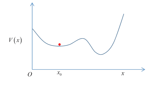
To simplify the equations, we’ll also move the $x$ origin to $x_0$, so

$$m\ddot{x}=-V^{″}\left(0\right)x=-kx,$$

replacing the second derivative with the standard “spring constant” expression.

This equation has solution

$$x=A\cos \left(\omega t+\delta \right),\text{ or }x=\mathrm{Re}\left(B{e}^{i\omega t}\right),B=A{e}^{i\delta },\omega =\sqrt{k/m}.$$

(This can, of course, also be derived from the Lagrangian, easily shown to be $L=\frac{1}{2}m{\dot{x}}^2-\frac{1}{2}m{\omega }^2{x}^2.$ )

Two Coupled Pendulums

We’ll take two equal pendulums, coupled by a light spring.  We take the spring restoring force to be directly proportional to the angular difference between the pendulums.  (This turns out to be a good approximation.)

For small angles of oscillation, we take the Lagrangian to be

$$L=\frac{1}{2}m{\ell }^2{\dot{\theta }}_1^2+\frac{1}{2}m{\ell }^2{\dot{\theta }}_2^2-\frac{1}{2}mg\ell {\theta }_1^2-\frac{1}{2}mg\ell {\theta }_2^2-\frac{1}{2}C{\left({\theta }_1-{\theta }_2\right)}^2.$$

Denoting the single pendulum frequency by ${\omega }_0$, the equations of motion are (writing ${\omega }_0^2=g/\ell ,k=C/m{\ell }^2$ , so $\left[k\right]=T^{-2}$ )

$$\begin{array}{l}{\ddot{\theta }}_1=-{\omega }_0^2{\theta }_1-k\left({\theta }_1-{\theta }_2\right)\\ {\ddot{\theta }}_2=-{\omega }_0^2{\theta }_2-k\left({\theta }_2-{\theta }_1\right).\end{array}$$

We look for a periodic solution, writing

$${\theta }_1\left(t\right)=A_1{e}^{i\omega t},{\theta }_2\left(t\right)=A_2{e}^{i\omega t},$$

 (The final physical angle solutions will be the real part.)

The equations become (in matrix notation):

$${\omega }^2\left(\begin{array}{c}{A}_1\\ A_2\end{array}\right)=\left(\begin{array}{cc}{\omega }_0^2+k& -k\\ -k& {\omega }_0^2+k\end{array}\right)\left(\begin{array}{c}{A}_1\\ A_2\end{array}\right).$$

Denoting the $2\times 2$ matrix by $M,$   

$M\overrightarrow{A}={\omega }^2\overrightarrow{A},\overrightarrow{A}=\left(\begin{array}{c}{A}_1\\ A_2\end{array}\right).$ 

This is an eigenvector equation, with ${\omega }^2$ the eigenvalue, found by the standard procedure:

$$\det \left(M-{\omega }^{2}I\right)=\left|\begin{array}{cc}{\omega }_0^2+k-{\omega }^2& -k\\ -k& {\omega }_0^2+k-{\omega }^2\end{array}\right|=0.$$

Solving, ${\omega }^2={\omega }_0^2+k\pm k,$ that is,

$${\omega }^2={\omega }_0^2,{\omega }^2={\omega }_0^2+2k.$$

The corresponding eigenvectors are $\left(1,1\right)$ and $\left(1,-1\right)$.

Normal Modes

The physical motion corresponding to the amplitudes eigenvector $\left(1,1\right)$ has two constants of integration (amplitude and phase), often written in terms of a single complex number, that is,

$$\left(\begin{array}{c}{\theta }_1\left(t\right)\\ {\theta }_2\left(t\right)\end{array}\right)=\left(\begin{array}{c}1\\ 1\end{array}\right)\mathrm{Re}B{e}^{i{\omega }_{0}t}=\left(\begin{array}{c}A\cos \left({\omega }_{0}t+\delta \right)\\ A\cos \left({\omega }_{0}t+\delta \right)\end{array}\right),B=A{e}^{i\delta }$$

with $A,\delta$ real.

Clearly, this is the mode in which the two pendulums are in sync, oscillating at their natural frequency, with the spring playing no role. 

In physics, this mathematical eigenstate of the matrix is called a normal mode of oscillation.  In a normal mode, all parts of the system oscillate at a single frequency, given by the eigenvalue.

The other normal mode,

$$\left(\begin{array}{c}{\theta }_1\left(t\right)\\ {\theta }_2\left(t\right)\end{array}\right)=\left(\begin{array}{c}1\\ -1\end{array}\right)\mathrm{Re}B{e}^{i{\omega }^{\prime }t}=\left(\begin{array}{c}A\cos \left({\omega }^{\prime }t+\delta \right)\\ -A\cos \left({\omega }^{\prime }t+\delta \right)\end{array}\right),B=A{e}^{i\delta }$$

where we have written ${\omega }^{\prime }=\sqrt{{\omega }_0^2+2k}$. Here the system is oscillating with the single frequency ${\omega }^{\prime }$, the pendulums are now exactly out of phase,  so when they part the spring pulls them back to the center, thereby increasing the system oscillation frequency.

The matrix structure can be clarified by separating out the spring contribution:

$$M=\left(\begin{array}{cc}{\omega }_0^2+k& -k\\ -k& {\omega }_0^2+k\end{array}\right)={\omega }_0^2\left(\begin{array}{cc}1& 0\\ 0& 1\end{array}\right)+k\left(\begin{array}{cc}1& -1\\ -1& 1\end{array}\right).$$

All vectors are eigenvectors of the identity, of course, so the first matrix just contributes ${\omega }_0^2$to the eigenvalue. The second matrix is easily found to have eigenvalues are 0,2, and eigenstates $\left(1,1\right)$ and $\left(1,-1\right)$.

Principle of Superposition

The equations of motion are linear equations, meaning that if you multiply a solution by a constant, that’s still a solution, and if you have two different solutions to the equation, the sum of the two is also a solution. This is called the principle of superposition. 

The general motion of the system is therefore

$$\begin{array}{l}{\theta }_1\left(t\right)=A{e}^{i{\omega }_{0}t}+B{e}^{i\sqrt{{\omega }_0^2+2k}t}\\ {\theta }_2\left(t\right)=A{e}^{i{\omega }_{0}t}-B{e}^{i\sqrt{{\omega }_0^2+2k}t}\end{array}$$

where it is understood that $A,B$ are complex numbers and the physical motion is the real part.

This is a four-parameter solution: the initial positions and velocities can be set arbitrarily, completely determining the motion.

Exercise:  begin with one pendulum straight down, the other displaced, both momentarily at rest.  Find values for $A,B$ and describe the subsequent motion.

Solution: At $t=0,$ the pendulums are at $A\pm B.$ Take $A=B=1.$ This ensures zero initial velocities too, since the physical parameters are the real parts of the complex solution, and at the initial instant the derivatives are pure imaginary.

The solution for the motion of the first pendulum is

${\theta }_1\left(t\right)=\cos {\omega }_{0}t+\cos {\left({\omega }_0^2+2k\right)}^{\frac{1}{2}}t=2\cos \frac{1}{2}\left({\left({\omega }_0^2+2k\right)}^{\frac{1}{2}}+{\omega }_0\right)t\cos \frac{1}{2}\left({\left({\omega }_0^2+2k\right)}^{\frac{1}{2}}-{\omega }_0\right)t$.

and for small $k$,

${\theta }_1\left(t\right)\cong 2\cos {\omega }_{0}t\cos \left(k/{\omega }_0\right)t.$ 

 Here the pendulum is oscillating at approximately ${\omega }_0$, but the second term sets the overall oscillation amplitude: it's slowly varying, going to zero periodically (at which point the other pendulum has maximum kinetic energy).

To think about:  What happens if the two have different masses?  Do we still get these beats -- can the larger pendulum transfer all its kinetic energy to the smaller?

Exercise: try pendulums of different lengths, hung so the bobs are at the same level, small oscillation amplitude, same spring as above.

Three Coupled Pendulums

Let’s now move on to the case of three equal mass coupled pendulums, the middle one connected to the other two, but they’re not connected to each other.

The Lagrangian is

$$L=\frac{1}{2}m{\ell }^2{\dot{\theta }}_1^2+\frac{1}{2}m{\ell }^2{\dot{\theta }}_2^2+\frac{1}{2}m{\ell }^2{\dot{\theta }}_3^2-\frac{1}{2}mg\ell {\theta }_1^2-\frac{1}{2}mg\ell {\theta }_2^2-\frac{1}{2}mg\ell {\theta }_3^2-\frac{1}{2}C{\left({\theta }_1-{\theta }_2\right)}^2-\frac{1}{2}C{\left({\theta }_3-{\theta }_2\right)}^2.$$

Putting ${\omega }_0^2=g/\ell ,k=C/m{\ell }^2$,

$$L=\frac{1}{2}{\dot{\theta }}_1^2+\frac{1}{2}{\dot{\theta }}_2^2+\frac{1}{2}{\dot{\theta }}_3^2-\frac{1}{2}{\omega }_0^2{\theta }_1^2-\frac{1}{2}{\omega }_0^2{\theta }_2^2-\frac{1}{2}{\omega }_0^2{\theta }_3^2-\frac{1}{2}k{\left({\theta }_1-{\theta }_2\right)}^2-\frac{1}{2}k{\left({\theta }_3-{\theta }_2\right)}^2.$$

The equations of motion are

$$\begin{array}{l}{\ddot{\theta }}_1=-{\omega }_0^2{\theta }_1-k\left({\theta }_1-{\theta }_2\right)\\ {\ddot{\theta }}_2=-{\omega }_0^2{\theta }_2-k\left({\theta }_2-{\theta }_1\right)-k\left({\theta }_2-{\theta }_3\right)\\ {\ddot{\theta }}_3=-{\omega }_0^2{\theta }_3-k\left({\theta }_3-{\theta }_2\right).\end{array}$$

Putting ${\theta }_i\left(t\right)=A_i{e}^{i\omega t}$, the equations can be written in matrix form

$$\left(\begin{array}{ccc}{\omega }_0^2+k& -k& 0\\ -k& {\omega }_0^2+2k& -k\\ 0& -k& {\omega }_0^2+k\end{array}\right)={\omega }_0^2\left(\begin{array}{ccc}1& 0& 0\\ 0& 1& 0\\ 0& 0& 1\end{array}\right)+k\left(\begin{array}{ccc}1& -1& 0\\ -1& 2& -1\\ 0& -1& 1\end{array}\right)$$

The normal modes of oscillation are given by the eigenstates of that second matrix.

The one obvious normal mode is all the pendulums swinging together, at the original frequency ${\omega }_0$, so the springs stay at the rest length and play no role. For this mode, evidently the second matrix has a zero eigenvalue, and eigenvector $\left(1,1,1\right)$.

The full eigenvalue equation is

$$\left|\begin{array}{ccc}1-\lambda & -1& 0\\ -1& 2-\lambda & -1\\ 0& -1& 1-\lambda \end{array}\right|=0,$$

that is,

${\left(1-\lambda \right)}^2\left(2-\lambda \right)-2\left(1-\lambda \right)=0=\left(1-\lambda \right)\left[\left(1-\lambda \right)\left(2-\lambda \right)-2\right]=\left(1-\lambda \right)\left({\lambda }^2-3\lambda \right),$

 so the eigenvalues are ${\lambda }_1=0,{\lambda }_2=1,{\lambda }_3=3$, with frequencies

$${\omega }_1^2={\omega }_0^2,{\omega }_2^2={\omega }_0^2+k,{\omega }_3^2={\omega }_0^2+3k.$$

  The normal mode eigenvectors satisfy

$$\left(\begin{array}{ccc}1-\lambda & -1& 0\\ -1& 2-\lambda & -1\\ 0& -1& 1-\lambda \end{array}\right)\left(\begin{array}{c}{A}_1\\ A_2\\ A_3\end{array}\right)=0.$$

They are $\left(1,1,1\right)/\sqrt{3},\left(1,0,-1\right)/\sqrt{2},\left(1,-2,1\right)/\sqrt{6}$, normalizing them to unity.

The equations of motion are linear, so the general solution is a superposition of the normal modes:

$$\left(\begin{array}{c}{\theta }_1\\ {\theta }_2\\ {\theta }_3\end{array}\right)=\frac{1}{\sqrt{3}}\left(\begin{array}{c}1\\ 1\\ 1\end{array}\right)\mathrm{Re}\left(C_1{e}^{i{\omega }_{1}t}\right)+\frac{1}{\sqrt{2}}\left(\begin{array}{c}1\\ 0\\ -1\end{array}\right)\mathrm{Re}\left(C_2{e}^{i{\omega }_{2}t}\right)+\frac{1}{\sqrt{6}}\left(\begin{array}{c}1\\ -2\\ 1\end{array}\right)\mathrm{Re}\left(C_3{e}^{i{\omega }_{3}t}\right).$$

Normal Coordinates

Landau writes $Q_{\alpha }=\mathrm{Re}{C}_{\alpha }{e}^{i{\omega }_{\alpha }t}$.  (Actually he brings in an intermediate variable ${\Theta }_{\alpha }$, but we'll skip that.) These “normal coordinates” can have any amplitude and phase, but oscillate at a single frequency ${\ddot{Q}}_{\alpha }=-{\omega }_{\alpha }^2{Q}_{\alpha }.$ 

The components of the above vector equation read:

$$\begin{array}{l}{\theta }_1=Q_1/\sqrt{3}+Q_2/\sqrt{2}+Q_3/\sqrt{6}\\ {\theta }_2=Q_1/\sqrt{3}-2Q_3/\sqrt{6}\\ {\theta }_3=Q_1/\sqrt{3}-Q_2/\sqrt{2}+Q_3/\sqrt{6}.\end{array}$$

It’s worth going through the exercise of writing the Lagrangian in terms of the normal coordinates:

recall the Lagrangian:

$$L=\frac{1}{2}{\dot{\theta }}_1^2+\frac{1}{2}{\dot{\theta }}_2^2+\frac{1}{2}{\dot{\theta }}_3^2-\frac{1}{2}{\omega }_0^2{\theta }_1^2-\frac{1}{2}{\omega }_0^2{\theta }_2^2-\frac{1}{2}{\omega }_0^2{\theta }_3^2-\frac{1}{2}k{\left({\theta }_1-{\theta }_2\right)}^2-\frac{1}{2}k{\left({\theta }_3-{\theta }_2\right)}^2.$$ 

Putting in the above expressions for the ${\theta }_{\alpha }$, after some algebra,

$$L=\frac{1}{2}\left[{\dot{Q}}_1^2-{\omega }_0^2{Q}_1^2\right]+\frac{1}{2}\left[{\dot{Q}}_2^2-\left({\omega }_0^2+k\right)Q_2^2\right]+\frac{1}{2}\left[{\dot{Q}}_3^2-\left({\omega }_0^2+3k\right)Q_3^2\right].$$

We’ve achieved a separation of variables.  The Lagrangian is manifestly a sum of three simple harmonic oscillators, which can have independent amplitudes and phases.  Incidentally, this directly leads to the action angle variables -- recall that for a simple harmonic oscillator the action $I=E/\omega ,$ and the angle is that of rotation in phase space.

Three Equal Pendulums Equally Coupled

What if we had a third identical spring connecting the two end pendulums (we could have small rods extending down so the spring went below the middle pendulum?

What would the modes of oscillation look like in this case?

Obviously, all three swinging together is still an option, the eigenvector $\left(1,1,1\right)$, corresponding to eigenvalue zero of the “interaction matrix” above.  But actually we have to extend that matrix to include the new spring -- it’s easy to check this gives the equation:

$$\left(\begin{array}{ccc}2-\lambda & -1& -1\\ -1& 2-\lambda & -1\\ -1& -1& 2-\lambda \end{array}\right)\left(\begin{array}{c}{A}_1\\ A_2\\ A_3\end{array}\right)=0.$$

The equation for the eigenvalues is easily found to be $\lambda {\left(\lambda -3\right)}^2=0.$ Putting $\lambda =3$ into the matrix yields the equation $A_1+A_2+A_3=0.$ This is telling us that any vector perpendicular to the all-swinging-together vector $\left(1,1,1\right)$ is an eigenvector. This is because the other two eigenvectors have the same eigenvalue, meaning that any linear combination of them also has that eigenvalue$—$this is a degeneracy. 

Think about the physical situation. If we set the first two pendulums swinging exactly out of phase, the third pendulum will feel no net force, so will stay at rest. But we could equally choose another pair.  And, the eigenvector $\left(1,-2,1\right)$ we found before is still an eigenvector: it's in this degenerate subspace, equal to $\left(1,-1,0\right)-\left(0,1,-1\right)$ .

 previous  home  next  PDF