previous  home  next  PDF

18. Driven Oscillator

Michael Fowler  (closely following Landau para 22)

Consider a one-dimensional simple harmonic oscillator with a variable external force acting, so the equation of motion is

$\ddot{x}+{\omega }^{2}x=F\left(t\right)/m,$ 

which would come from the Lagrangian

$L=\frac{1}{2}m{\dot{x}}^2-\frac{1}{2}k{x}^2+xF\left(t\right).$ 

(Landau “derives” this as the leading order non-constant term in a time-dependent external potential.)

The general solution of the differential equation is $x=x_0+x_1$ , where $x_0=a\cos \left(\omega t+\alpha \right)$ , the solution of the homogeneous equation, and $x_1$ is some particular integral of the inhomogeneous equation.

An important case is that of a periodic driving force $F\left(t\right)=f\cos \left(\gamma t+\beta \right).$  A trial solution $x_1\left(t\right)=b\cos \left(\gamma t+\beta \right)$ yields $b=f/m\left({\omega }^2-{\gamma }^2\right)$ so

$$x\left(t\right)=a\cos \left(\omega t+\alpha \right)+\frac{f}{m\left({\omega }^2-{\gamma }^2\right)}\cos \left(\gamma t+\beta \right).$$  But what happens when $\gamma =\omega$?  To find out, take part of the first solution into the second, that is,

$$x\left(t\right)=a^{\prime }\cos \left(\omega t+{\alpha }^{\prime }\right)+\frac{f}{m\left({\omega }^2-{\gamma }^2\right)}\left[\cos \left(\gamma t+\beta \right)-\cos \left(\omega t+\beta \right)\right].$$  The second term now goes to $0/0$ as $\gamma \to \omega$ , so becomes the ratio of its first derivatives with respect to $\omega$ (or, equivalently, $\gamma$ ).

$$x\left(t\right)=a^{\prime }\cos \left(\omega t+{\alpha }^{\prime }\right)+\frac{f}{2m\omega }t\sin \left(\omega t+\beta \right).$$ The amplitude of the oscillations grows linearly with time.  Obviously, this small oscillations theory will crash eventually.

But what if the external force frequency is slightly off resonance?

Then (real part understood)

$$x=A{e}^{i\omega t}+B{e}^{i\left(\omega +\epsilon \right)t}=\left(A+B{e}^{i\epsilon t}\right)e^{i\omega t},A=a{e}^{i\alpha },B=b{e}^{i\beta }$$with $a,b,\alpha ,\beta$ real.

The wave amplitude squared

$$C^2={\left|A+B{e}^{i\epsilon t}\right|}^2=a^2+b^2+2ab\cos \left(\epsilon t+\beta -\alpha \right).$$We’re seeing beats, with beat frequency $\epsilon .$ Note that if the oscillator begins at the origin, $x\left(t=0\right)=0,$ then $A+B=0$ and the amplitude periodically goes to zero, this evidently only occurs when $\left|A\right|=\left|B\right|.$

Energy is exchanged back and forth with the driving external force.

More General Energy Exchange

We’ll derive a formula for the energy fed into an oscillator by an arbitrary time-dependent external force.

The equation of motion can be written

$$\frac{d}{dt}\left(\dot{x}+i\omega x\right)-i\omega \left(\dot{x}+i\omega x\right)=\frac{1}{m}F\left(t\right)$$and defining $\xi =\dot{x}+i\omega x,$ this is

$d\xi /dt-i\omega \xi =F\left(t\right)/m.$

This first-order equation integrates to

$$\xi \left(t\right)=e^{i\omega t}\left({\displaystyle \underset{0}{\overset{t}{\int }}\frac{1}{m}F\left(t^{\prime }\right)e^{-i\omega t^{\prime }}d{t}^{\prime }+{\xi }_0}\right)$$The energy of the oscillator is

$$E=\frac{1}{2}m\left({\dot{x}}^2+{\omega }^2{x}^2\right)=\frac{1}{2}m{\left|\xi \right|}^2$$So if we drive the oscillator over all time, with beginning energy zero,

$$E=\frac{1}{2m}{\left|{\displaystyle \underset{-\infty }{\overset{\infty }{\int }}F\left(t\right)e^{-i\omega t}dt}\right|}^2.$$This is equivalent to the quantum mechanical time-dependent perturbation theory result: $\xi ,{\xi }^{\ast }$ are equivalent to the annihilation and creation operators.

Damped Driven Oscillator

The linear damped driven oscillator:

$\ddot{x}+2\lambda \dot{x}+{\omega }_0^{2}x=\left(f/m\right)e^{i\Omega t}.$

(Following Landau’s notation here$—$note it means the actual frictional drag force is $2\lambda m\dot{x}$ )

Looking near resonance for steady state solutions at the driving frequency, with amplitude $b$, phase lag $\delta$, that is, $x\left(t\right)=b{e}^{i\left(\Omega t+\delta \right)}$, we find

$$b{e}^{i\delta }\left(-{\Omega }^2+2i\lambda \Omega +{\omega }_0^2\right)=\left(f/m\right).$$For a near-resonant driving frequency $\Omega ={\omega }_0+\epsilon$, and assuming the damping to be sufficiently small that we can drop the $\epsilon \lambda$ term along with ${\epsilon }^2$, the leading order terms give

$b{e}^{i\delta }=-f/2m\left(\epsilon -i\lambda \right){\omega }_0$,

so the response, the dependence of amplitude of oscillation on frequency, is to this accuracy

$$b=\frac{f}{2m{\omega }_0\sqrt{{\left(\Omega -{\omega }_0\right)}^2+{\lambda }^2}}=\frac{f}{2m{\omega }_0\sqrt{{\epsilon }^2+{\lambda }^2}}.$$(We might also note that the resonant frequency is itself lowered by the damping, but this is another second-order effect we ignore here.)

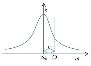
The rate of absorption of energy equals the frictional loss. The friction force $2\lambda m\dot{x}$ on the mass moving at $\dot{x}$ is doing work at a rate:

$2\lambda m\overline{{\dot{x}}^2}=\lambda m{b}^2{\Omega }^2.$

The half width of the resonance curve as a function of driving frequency $\Omega$ is given by the damping.  The total area under the curve is independent of damping. 

For future use, we’ll write the above equation for the amplitude as   $$b^2\left({\epsilon }^2+{\lambda }^2\right)=\frac{f^2}{4m^2\omega {}_0^2}.$$

My Applet of a Driven Damped Oscillator is available here, all the parameters can be adjusted to explore response.

The Excel spreadsheet for a driven damped oscillator I showed in class can be downloaded here.

 previous  home  next  PDF