2. Boundary Conditions at Surfaces
Introduction
Following Jackson (we’ve got to section 1.5) we’ll look at interfaces between media. It’s a slight puzzle why Jackson does this now, he assumes you’ve seen the integral form of Maxwell’s equations in an undergraduate course, and we’ll go along. First we’ll look at field discontinuities on going say from air into glass, then we’ll review the closely related problem of field discontinuity from a surface charge layer, finally we’ll examine a dipole layer, which we’ll need shortly.
Field Discontinuities at an Interface between Media
Imagine a locally flat interface between two uniform materials having different (We don’t take the more general tensor form.)
In this section, we’ll assume there is no charge or current on the interface.
 We’re
interested in how the electric and magnetic field vectors change on crossing
from one medium to the other.
We’re
interested in how the electric and magnetic field vectors change on crossing
from one medium to the other.
First we’ll examine the change in the normal to the surface components of the fields.
We find this by using the first two Maxwell equations (in integral form):
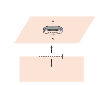
The trick is to integrate the vector fields over the complete surface of a vanishingly small pillbox, very thin, having its circular flat surfaces one in each medium.
The area of the cylindrical sides goes to zero in the limit we’re interested in, and the pillbox is so small we can take the field constant over the range of the integral, so, (for no charge at the boundary surface between the media)
This is often written as
Note that since this is not the same as !
The tangential components can be found using the other two Maxwell equations,
Recall the left-hand sides are integrals around loops, the right-hand sides integrals over surfaces spanning the loops.
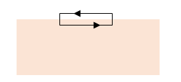 We choose as
loops of integration tiny rectangles with long sides parallel to the surface
and very close but on opposite sides, and much shorter sides perpendicular to
the surface. The contribution to the loop integral from these shorter sides
vanishes in the thin limit, and the result is
We choose as
loops of integration tiny rectangles with long sides parallel to the surface
and very close but on opposite sides, and much shorter sides perpendicular to
the surface. The contribution to the loop integral from these shorter sides
vanishes in the thin limit, and the result is
It is straightforward to generalize to the case where the surface has nonzero charge density and/or current density:
the vector being the surface current density.
Electric Field Discontinuity across a Charged Surface
This seems a good place to add a very similar scenario: a flat plane of charge in vacuum, charge density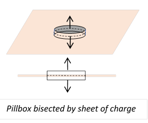 coul/m2. Assuming no other charges are present, the
electric fields on the two sides of the plane will be uniform, perpendicular to
the plane and in opposite directions on the two sides, both pointing outwards
if the plane is positively charged. The magnitude of the fields is easily found
by using Gauss’ law for a pillbox shape, two round flat sides of area parallel to the sheet of charge and on
opposite sides. The cylindrical side is
taken to go to zero in the limit. The enclosed charge is the flat sides contribute to the Gaussian integral, so
coul/m2. Assuming no other charges are present, the
electric fields on the two sides of the plane will be uniform, perpendicular to
the plane and in opposite directions on the two sides, both pointing outwards
if the plane is positively charged. The magnitude of the fields is easily found
by using Gauss’ law for a pillbox shape, two round flat sides of area parallel to the sheet of charge and on
opposite sides. The cylindrical side is
taken to go to zero in the limit. The enclosed charge is the flat sides contribute to the Gaussian integral, so
There is a discontinuity in the normal component (the only one present in this example) of the electric field.
Let’s think a little further concerning this discontinuity. Imagine we’re looking in the neighborhood of a point which is a tiny distance from the plane. If we now move through the plane, it experiences this discontinuity in field.
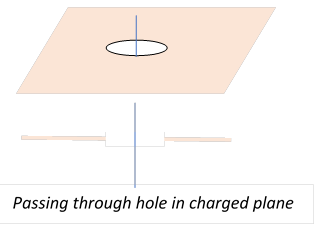 Now,
mentally split the field in this small region into two contributions, that from
charge within a small circle around where passed through the plane, the other
contribution from the (further away) rest of the plane, that is, from a plane
with a small hole in it, and we’re looking at the electric field on going
through the middle of the hole, along a line perpendicular to the plane. The electric field from this rest of the
plane has to be continuous along this lineso the discontinuity is generated entirely
by the very local charge distribution.
Now,
mentally split the field in this small region into two contributions, that from
charge within a small circle around where passed through the plane, the other
contribution from the (further away) rest of the plane, that is, from a plane
with a small hole in it, and we’re looking at the electric field on going
through the middle of the hole, along a line perpendicular to the plane. The electric field from this rest of the
plane has to be continuous along this lineso the discontinuity is generated entirely
by the very local charge distribution.
It follows that for any reasonably smooth surface, not necessarily plane, having in general varying charge density, there will be a discontinuity in the normal component of the electric field of magnitude depending on the local charge on passing through it.
Electric Potential Change across a Dipole Surface
Dipole surfaces are certainly less common, although they do exist in biological systems. But they also come up in some important mathematics, as we’ll see in a while, so this is worth thinking through.
The Dipole
Before analyzing the dipole surface, let's remind ourselves about a single dipole. The dipole is defined as the limit of two equal and opposite charges , separated by a small displacement in the limit under the condition that is held constant.
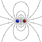
(This drawing from here.)
The vector quantity is called the dipole moment. The vector points from the negative charge to the positive charge.
The potential from a dipole at the origin is
The electric field
where as usual means a vector of unit length.
Potential Discontinuity across a Dipole Sheet
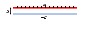 We
first consider a flat sheet of uniform strength dipole, meaning a sheet with
uniform charge surface density coul/m2, separated by a distance from a sheet oppositely charged, in the limit holding ,
the dipole surface density, constant.
We
first consider a flat sheet of uniform strength dipole, meaning a sheet with
uniform charge surface density coul/m2, separated by a distance from a sheet oppositely charged, in the limit holding ,
the dipole surface density, constant.
We proved above that for a single uniform sheet of charge the electric fields above and below were taking that for the (upper) positive sheet of the dipole, the negative sheet will contribute fields also extending throughout space, so the fields will exactly cancel except between the sheets, where
The potential difference between the sheets .
On crossing a uniform sheet of dipole there is a discontinuity in the potential equal to dipole strength
Electrostatic Potential from a Dipole Layer
Assume an arbitrary surface having uniform dipole strength meaning that each increment of area has dipole strength
The electrostatic potential at the origin from the surface increment is, from the dipole potential formula in the previous section,
since is the projection of the area on to a plane perpendicular to equal to .
Therefore, at a point, the potential from the whole dipole surface equals the solid angle subtended.
Exercise: Take a single dipole to be a tiny disc, and visualize the solid angle subtended at different points in spaceshow this reproduces the dipole potential found above.
Closed Uniform Dipole Layer
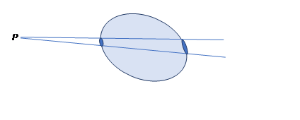 Taking
a point P outside the surface, since
each increment of surface contributes to the potential at P proportional to the
solid angle subtended (and remember the sign!) the total closed surface will
contribute zero potentialcancellation
between the increments shown, which subtend the same solid angle at P, but clearly with opposite signs. On the other hand, if P is inside the surface,
the contributions all have the same sign, so the potential at all points inside
is the same, equal to in agreement with the potential discontinuity
given above.
Taking
a point P outside the surface, since
each increment of surface contributes to the potential at P proportional to the
solid angle subtended (and remember the sign!) the total closed surface will
contribute zero potentialcancellation
between the increments shown, which subtend the same solid angle at P, but clearly with opposite signs. On the other hand, if P is inside the surface,
the contributions all have the same sign, so the potential at all points inside
is the same, equal to in agreement with the potential discontinuity
given above.