previous  index  next 

24. Electric Field of a Charged Needle

    Michael Fowler, UVa

Introduction and Coordinates

By a needle we mean a very thin straight piece of conducting wire. This problem is somewhat similar to the charged conducting thin disc we just discussed, and indeed the same elliptic coordinates are appropriate, except that in this case we need the prolate rather than the oblate ellipsoids.  

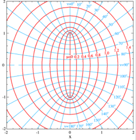
Glancing at the plot (from Wikipedia) it is evident that the central $\mu =0$ line on the $z$ axis will represent the needle (an equipotential of course) and that the other ellipsoids of constant $\mu$ will be equipotentials.  (Just as for the disc, this is an axially symmetric three-dimensional potential problem, we are looking in the diagram at a cross section corresponding to constant axial angle.)

For now, we’ll think of the needle as the limit of an extremely thin prolate ellipsoid, rather than say, the limit of a circular cylinder with flat ends as the radius goes to zero. Does that matter? The difference is small, as we’ll see later.  

Prolate spheroidal coordinates differ from the oblate in having cosh and sinh interchanged, also $\cos \nu \text{ and }\sin \nu .$ That is,

$\begin{array}{l}x=a\sinh \mu \sin \nu \cos \phi ,\\ y=a\sinh \mu \sin \nu \sin \phi ,\\ z=a\cosh \mu \cos \nu .\end{array}$

The equipotentials are the ellipsoids ( ${\rho }^2=x^2+y^2$ )

$$\frac{{\rho }^2}{a^2{\sinh }^2\mu }+\frac{z^2}{a^2{\cosh }^2\mu }={\sin }^2\nu +{\cos }^2\nu =1.$$

The wire is along $\mu =0,$ the central segment of the $z$ axis, from $a$ to $-a.$

The scaling factors and derivation of the Laplacian are as for the disc, with the trivial adjustments mentioned above, and we find

$$\begin{array}{l}{\nabla }^2\Phi =\frac{1}{a^2\left({\sinh }^2\mu +{\sin }^2\nu \right)}\left[\frac{1}{\sinh \mu }\frac{\partial }{\partial \mu }\left(\sinh \mu \frac{\partial \Phi }{\partial \mu }\right)+\frac{1}{\sin \nu }\frac{\partial }{\partial \nu }\left(\cos \nu \frac{\partial \Phi }{\partial \nu }\right)\right]\\ +\frac{1}{a^2{\sinh }^2\mu {\sin }^2\nu }\frac{{\partial }^2\Phi }{\partial {\phi }^2}.\end{array}$$

We’re taking the potential to be a function of $\mu$ only, so

$$\frac{\partial }{\partial \mu }\left(\sinh \mu \frac{\partial \Phi }{\partial \mu }\right)=0,\text{ so }\frac{\partial \Phi }{\partial \mu }=\frac{\text{const}\text{.}}{\sinh \mu }=\frac{{\Phi }_0}{\sinh \mu }.$$

Note first that on the “equatorial” plane $z=0,\rho =a\sinh \mu ,$ and close to the wire ( $\mu \to 0$ ), we can take $\rho \cong a\mu$ to give $\partial \Phi /\partial \rho \propto 1/\rho ,$ the expected logarithmic potential, that from an infinite wire.

Doing the integral,

$\Phi ={\Phi }_0\ln \left|\tanh \frac{\mu }{2}\right|+\text{ const}\text{.,}$

and we’ll fix the constant by taking the potential zero at infinity.  For large distances, $\mu$ is also large, in fact for large $r^2={\rho }^2+z^2,$

$r\cong \frac{1}{2}a{e}^{\mu }.$

In this limit $\tanh \left(\mu /2\right)\cong 1-2e^{-\mu },$ so far away, matching our expression to the known result for $r\gg a,$

$\begin{array}{l}\Phi \cong {\Phi }_0\left(-2e^{-\mu }\right)=-{\Phi }_0\frac{a}{r}=-\frac{Q}{4\pi {\epsilon }_{0}r},\\ \text{so }{\Phi }_0=\frac{Q}{4\pi {\epsilon }_{0}a}.\end{array}$

where $Q$ is the total charge on the needle (which has length $2a$ ).

Checking this for small $\rho$ at $z=0,$ for an infinite line charge of linear density $\lambda ,$ $2\pi \rho E=\lambda /{\epsilon }_0=Q/2a{\epsilon }_0,$ so  $E=Q/4\pi {\epsilon }_{0}a\rho ={\Phi }_0/\rho ,$ the value found above.

The capacitance $C$ of a thin prolate needle is defined by $\Phi =Q/C.$  From $\Phi ={\Phi }_0\ln \left|\tanh \frac{\mu }{2}\right|$ and $\rho \cong a\mu ,$ the surface potential for equatorial radius $b$ is to leading order ${\Phi }_0\left|\ln \left(b/2a\right)\right|,$ so the capacitance

$$C\cong \frac{4\pi {\epsilon }_{0}a}{\ln \left(2a/b\right)}.$$

An Apparent Paradox

What about the charge distribution along the line?  In the above discussion, we’ve implicitly assumed it’s uniform.  But from the map of equipotentials, the needle is all at the same potential, we’ve said it’s a conductor.  So wouldn’t you expect the charges on the needle, repelling each other, to pile up somewhat at the ends? If we take the limit of a thin prolate ellipsoid, the answer turns out to be no. Recall the way we found the charge distribution on a disc in the previous lecture by projecting down from a uniformly charged spherical surface to the equatorial plane, and finding that the electric fields in the plane of the disc from projections of opposite parts of the sphere exactly balanced, as they had for the spherical distribution itself, so there was no field tending to rearrange the charge density in the disc.  We can go through exactly the same argument, projecting from a uniformly charged sphere onto our thin ellipsoid as it becomes a line. The point is that slicing a sphere perpendicular to the axis, uniformly thick slices have the same surface area, so projecting the uniformly charged spherical surface onto the axis gives a uniform charge distribution. Clearly the geometry of the ellipsoid is crucial: the electric field, and hence the surface charge density, is higher at the ends. (The actual charge distribution on the ellipsoid can be found by projecting back from the line, using that along an ellipse $xdx/a^2=-ydy/b^2$ so incremental distance $ds=dx\left(b^2/y\right)\sqrt{\left(x^2/a^4\right)+\left(y^2/b^4\right)}.$ )

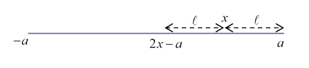
Still, this is difficult to believe (although the projection argument is valid).  Maxwell himself called it a paradox in 1877 (but added that Green had figured it out in 1832).  Here’s Maxwell’s reasoning: consider what repulsive forces from the rest of the charge distribution are felt by charge in an increment $\Delta x$ at a point $x$ (not of course at the center of the needle).   Assuming first a uniform distribution, total charge $Q=2a{\lambda }_0,$ the repulsion from charges between $x$ and the nearer end will clearly be balanced by that from charges up to an equal distance $\mathcal{l}$ the other way (see figure), but the rest of the charges to the left will surely push the charge in the interval $\Delta x$ to the right, presumably leading to a new distribution peaked at the ends. What’s wrong with this assertion?

One way to explore what might be wrong is to discretize: we’ll replace the charge distribution by a large number $N$ of equal charges $q=Q/N=2a{\lambda }_0/N,$ initially equally spaced.  We know they will rearrange from the argument just given$—$but by how much?  And what happens when $N\to \infty ?$

Let us focus on a single charge $q$ at the point $x.$ It will feel a force from the unbalanced charge on the left in the figure above, to leading order (meaning we take the charge distribution here to be ${\lambda }_0$ )

$F=q{\displaystyle \underset{-a}{\overset{2x-a}{\int }}\frac{{\lambda }_{0}dy}{{\left(y-x\right)}^2}=q{\lambda }_0\left[\frac{1}{x-a}+\frac{1}{x+a}\right]=\frac{2q{\lambda }_{0}x}{x^2-a^2}}.$

What is balancing this force? Think now of the local discretized distribution, first imagine it as equal charges $q=Q/N$ separated by equal distances $\delta =2a/N.$ We see immediately that the inverse square repulsion forces $q^2/{\delta }^2$ between nearest neighbors are each of order 1, whereas the force we are trying to balance is of order $1/N$!   This means that the forces from the two nearest neighbors can balance the faraway charges if their distances from our charge differ by an amount of order $\delta /N=2a/N^2.$ Of course, there are also contributions from further neighbors, and it turns out they’re important, but first as a toy exercise, let’s just balance the force above with unbalanced nearest neighbors. Of course the spacing must be varying, in other words $d\lambda \left(x\right)/dx\ne 0,$ since $\lambda \left(x\right)=q/\delta \left(x\right)$ and for given $N,q$ is constant.

We’ll take the nearest neighbor contributions to be

$\frac{q^2}{{\left(\delta -\frac{1}{2}\epsilon \right)}^2}-\frac{q^2}{{\left(\delta +\frac{1}{2}\epsilon \right)}^2}=\frac{q^2}{{\delta }^2}\left(1-1+\frac{2\epsilon }{\delta }\right)=\frac{2q^2\epsilon }{{\delta }^3}=-2q\frac{d\lambda }{dx}.$

This gives a simple differential equation for the density,

$\frac{d\lambda }{dx}={\lambda }_0\left[\frac{1}{x-a}+\frac{1}{x+a}\right]\text{(?)}$

and we see $\lambda \left(x\right)$ has logarithmic singularities at the ends.  But it’s wrong$—$we should have included further pairs of neighbors.  

Consider the next nearest neighbors: they will contribute

$\frac{q^2}{{\left(2\delta -2\epsilon \right)}^2}-\frac{q^2}{{\left(2\delta +2\epsilon \right)}^2}=\frac{q^2}{{\left(2\delta \right)}^2}\left(1-1+\frac{4\epsilon }{\delta }\right)=\frac{q^2\epsilon }{{\delta }^3},$ 

and the next ones

$\frac{q^2}{{\left(3\delta -\frac{9}{2}\epsilon \right)}^2}-\frac{q^2}{{\left(3\delta +\frac{9}{2}\epsilon \right)}^2}=\frac{q^2}{{\left(3\delta \right)}^2}\left(1-1+\frac{6\epsilon }{\delta }\right)=\frac{2q^2\epsilon }{3{\delta }^3},$

 so the correction to using just the nearest neighbors is a factor $\left(1+\frac{1}{2}+\frac{1}{3}+\dots \right),$ in other words, $\ln N$ where $N$ is some cutoff, such as the end of the line.  This means that the log singularities we found at the ends are suppressed by this factor, giving in the $N\to \infty$ limit a uniform distribution.  The approach to uniformity is very slow, going as $\ln N\sim \ln \left(a/\delta \right)$.  This is reminiscent of another approach, finding the line as a limit of a cylinder of length $2a$ and diameter $2b,$ where the corresponding parameter is of order $\ln \left(a/b\right).$

Another point: doesn’t Maxwell’s “lack of balance” argument contradict our earlier claim that you can project down from a spherical surface to the axis and corresponding elements of surface charge still balance after this projection?  But it’s a bit different: the balancing charges on the spherical surface are not in general equal, nor are their projections to the axis. Maxwell was balancing equal charge increments at equal distances.  Hmm.

Limit of a Thin Cylinder

The above analysis regarding the wire as the limit of a thin ellipsoid is mathematically exact, but what about the more practical limit, a very thin cylindrical wire? This has to be treated numerically, using variational methods. In fact, it is treated in a series of article in the American Journal of Physics by, yes, Jackson and Griffiths, in 2001. They expressed surprise that no-one had analyzed it previously, but in fact, as they later discovered to their chagrin, Maxwell had, and his approximation was very close to their final result.  (See Jackson, J. (2002). Charge density on a thin straight wire: The first visit. - AMER J PHYS. 70. 10.1119/1.1432973.)  The physically interesting result is how very slowly the uniform limit is approached as the radius tends to zero (logarithmically). And, the leading term in the capacitance is just that for the very thin ellipsoid found above, corrections being again logarithmic.

Historical Footnote: Green’s Proof that Equipotentials for a Line of Charge Are Ellipsoids

A very elegant proof, from Green in 1828  (Ferrers, p 329):

Suppose there is a uniform line of charge from A to B.  Take an arbitrary point P, and draw a circle in the plane PAB, center P, touching the line AB of charge, radius $a.$

Consider the force on a unit charge at P from the increment of charge on the line in angular interval $d\theta$ (see diagram).

 

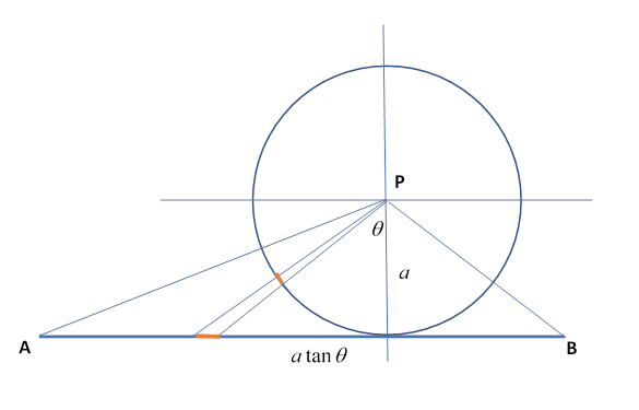
For charge density $\lambda ,$ the charge is  $\lambda a{\sec }^2\theta d\theta$ and the distance from P is $a\sec \theta ,$ so the electric field at P from this increment is $\lambda ad\theta /a^2,$ the same as that from the corresponding increment of the circle, if the circle had uniform charge distribution $\lambda .$

Therefore, the electric field at P from the line of charge is the same as that from a uniform linear charge distribution on the segment of the circle between the lines PA and PB. Hence the field is directed along the bisector of the angle APB, and so the equipotential, perpendicular to this, makes equal angles with PA and PB, so a ray originating at A would be reflected to B.

This means that the equipotential is an increment of an ellipse with foci at A and B.

previous  index  next