previous  index  next 

38  Maxwell’s Equations

    Michael Fowler, UVa

Pre-Maxwell

First, the pre-Maxwell equations$—$the story so far (excluding polarization and magnetization phenomena):

There are two so-called "homogeneous" equations, meaning they're purely field equations, no mention of charges and currents:

$$\begin{array}{c}\overrightarrow{\nabla }\cdot \overrightarrow{B}=0,\\ \overrightarrow{\nabla }\times \overrightarrow{E}+\frac{\partial \overrightarrow{B}}{\partial t}=0.\end{array}$$  The first equation states there are no magnetic monopoles, the second is Faraday's Law of Induction.

Then there are two equations stating how the fields arise from charge and current distributions:

$\begin{array}{c}\overrightarrow{\nabla }\cdot \overrightarrow{E}=\frac{\rho }{{\epsilon }_0},\\ \overrightarrow{\nabla }\times \overrightarrow{B}={\mu }_0\overrightarrow{j},\end{array}$

that last one being Ampère's Law.

What Maxwell added…

Maxwell's crucial contribution was the realization that the Ampere's law equation cannot be correct for time-dependent currents and charges.

Feynman gives a nice example of where Ampere's rule goes wrong.  Consider a large volume of uniform, conducting jello (having the same dielectric and magnetic properties as the vacuum).

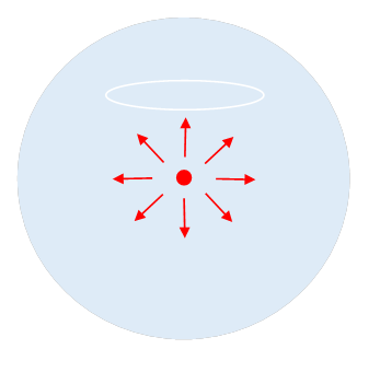  Inject with a slender needle a small spherical blob of charge in the middle.  The charge will disperse, and if we’ve kept the spherical symmetry successfully, current will go out equally in all directions. Now imagine a circular path like a halo placed above the central point where all the charge began. Current will be flowing through this halo. From Ampere's law, therefore, the line integral of the magnetic field around this circular halo must be nonzero.

But the current distribution is spherically symmetric$—$and therefore so must be any magnetic field it generates. However, no such magnetic field can exist!  It would have nonzero divergence. The actual magnetic field must therefore be exactly zero, and Ampere's law cannot be valid.

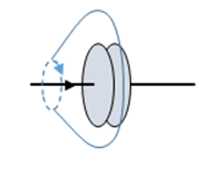
Another way to see Ampere's law can't be right for a time-dependent situation is to take the standard circle contour around a wire, giving $B={\mu }_{0}J/2\pi r,$ and recall this will hold even if the surface spanning the circle (to get from ${\displaystyle \int \overrightarrow{\nabla }\times \overrightarrow{B}\cdot d\overrightarrow{a}}$ to ${\displaystyle \underset{C}{\oint }\overrightarrow{B}\cdot d\overrightarrow{\ell }}$ ) is distorted, the wire will still go through the surface (possibly more than once, but an odd number of times). 

This reasoning fails, however, if the wire is charging a capacitor, and the surface can be slipped between the plates.  In that case, no current passes through the surface.

  These two examples have a common feature: in both cases, there is a local changing charge density, and therefore a changing electric field.  In the case of the parallel plate capacitor, we can be quantitative: take the plates close together, say the charge at some instant is $Q\left(t\right)$ the charging current $J=dQ/dt.$ 

The electric field penetrating the surface spanning the loop, but now passing between the capacitor plates,  is ${\displaystyle \int \overrightarrow{E}\cdot d\overrightarrow{a}=Q\left(t\right)/{\epsilon }_0.}$

 Hence

$$J=\frac{dQ}{dt}={\epsilon }_0{\displaystyle \underset{S}{\int }\frac{\partial \overrightarrow{E}}{\partial t}}\cdot d\overrightarrow{a}.$$  Therefore, to generalize Ampère's magnetostatic law to take care of this dynamical situation, it is apparent that the total rate of change of electric field through the surface has to be taken as equivalent to an electric current through the surface.

So, at least for this example, we find

$${\displaystyle \underset{S}{\int }\left({\mu }_0\overrightarrow{j}+{\mu }_0{\epsilon }_0\frac{\partial \overrightarrow{E}}{\partial t}\right)}\cdot d\overrightarrow{a}={\displaystyle \underset{C}{\oint }\overrightarrow{B}\cdot d\overrightarrow{\ell }}$$  or equivalently

$$\overrightarrow{\nabla }\times \overrightarrow{B}={\mu }_0\overrightarrow{j}+{\mu }_0{\epsilon }_0\frac{\partial \overrightarrow{E}}{\partial t}.$$  Maxwell called ${\epsilon }_0\partial \overrightarrow{E}/\partial t$ the "displacement current". 

The origin of this term is the behavior of dielectrics in varying electric fields: as the electric field acting on a dielectric increases, the molecular charge separation increases, this process is equivalent to a current (since opposite charges move in opposite directions) during the period the field strength is changing.  Maxwell imagined something similar was going on even in the vacuum, hence the term.  We don't think of it that way anymore (for the vacuum), but the term has stuck.

The above exercises are interesting and worthwhile (I hope), but really it should have been clear from the beginning that Ampere's law could not possibly be correct if charge densities are changing: since $\overrightarrow{\nabla }\cdot \overrightarrow{\nabla }\times \overrightarrow{B}\equiv 0,$ it would follow that $\overrightarrow{\nabla }\cdot \overrightarrow{j}\equiv 0,$ and hence from charge conservation $\partial \rho /\partial t\equiv 0,$ charge density staying constant.  Reassuringly, adding the displacement current term gives

$$\overrightarrow{\nabla }\cdot \overrightarrow{j}=-\frac{\partial }{\partial t}\overrightarrow{\nabla }\cdot {\epsilon }_0\overrightarrow{E}=-\frac{\partial \rho }{\partial t}.$$  The extended Ampere equation including the displacement current was Maxwell’s contribution, and it revolutionized electromagnetic theory: with this term, and only with this term, the equations predicted the possibility of waves, and led to the first real understanding of the nature of light.

To summarize, we now have the complete set of Maxwell's equations (in vacuum):

$$\begin{array}{c}\overrightarrow{\nabla }\cdot \overrightarrow{B}=0,\overrightarrow{\nabla }\times \overrightarrow{E}+\frac{\partial \overrightarrow{B}}{\partial t}=0,\\ \overrightarrow{\nabla }\cdot \overrightarrow{E}=\frac{\rho }{{\epsilon }_0},\overrightarrow{\nabla }\times \overrightarrow{B}={\mu }_0\overrightarrow{j}+{\mu }_0{\epsilon }_0\frac{\partial \overrightarrow{E}}{\partial t}.\end{array}$$ 

How the Displacement Current Makes Waves

We know, of course, that oscillating charges and currents emit waves, a large part of our civilization depends on it.  How do the fields far away from the source behave?  The equations are

$$\begin{array}{c}\overrightarrow{\nabla }\times \overrightarrow{B}={\mu }_0{\epsilon }_0\frac{\partial \overrightarrow{E}}{\partial t},\\ \overrightarrow{\nabla }\times \overrightarrow{E}=-\frac{\partial \overrightarrow{B}}{\partial t}.\end{array}$$  Taking the curl of either equation, and using curl curl = grad div $–$ del squared, and that both fields have zero divergence (away from sources), it follows immediately that both fields obey the wave equation,

$$\begin{array}{l}{\nabla }^2\overrightarrow{E}-\frac{1}{c^2}\frac{{\partial }^2\overrightarrow{E}}{\partial t^2}=0,\\ {\nabla }^2\overrightarrow{B}-\frac{1}{c^2}\frac{{\partial }^2\overrightarrow{B}}{\partial t^2}=0,\end{array}$$  with $c^2=1/{\mu }_0{\epsilon }_0$. 

To see this describes wave-type behavior, just look at the equation for the $x$ component of the electric field:

$${\partial }^2{E}_x/\partial x^2-\left(1/c^2\right){\partial }^2{E}_x/\partial t^2=0.$$  This is satisfied by any function of the form $f\left(x-ct\right)$ or $f\left(x+ct\right),$ an electric field configuration propagating at speed $c$ in the $\pm x$ direction, without changing its shape.

This was the result that convinced Maxwell his analysis was correct$—$in modern terminology, ${\mu }_0$ is fixed at $4\pi \cdot {10}^{-7},$ then a magnetostatic experiment is necessary to find the unit current and therefore unit charge, finally an electrostatic experiment determines ${\epsilon }_0.$

The crucial point is that these are static experiments, yet with Maxwell's theory they predict a wave velocity exactly equal to the measured velocity of light!  This was the first insight into the real nature of light.

General Solution of Maxwell's Equations

We’ve just seen that away from charges and currents, Maxwell’s equations have wave solutions. But how, exactly, do these waves get generated by moving charges and currents? In electrostatics (and magnetostatics) the key to finding the fields turned out to be the introduction of potentials, which obeyed differential equations having the charges (and currents) as source terms. The equations were then solvable by Green’s function methods. We’ll follow the same strategy here. Since we now have both electric and magnetic fields, and time dependence, this is obviously more technically challenging! But it works.

Brief Recap of Electrostatic and Magnetostatic Tricks: Potentials

In electrostatics, we had two equations, $\overrightarrow{\nabla }\times \overrightarrow{E}=0,\overrightarrow{\nabla }\cdot E=\rho /{\epsilon }_0.$ The fruitful approach we used was to realize that the first equation is solved by the gradient of any scalar function, called here the potential, $\overrightarrow{E}=-\overrightarrow{\nabla }\phi ,$ by analogy with gravitational potential, the change in $\phi$ between any two points being ${\displaystyle {\int }_A^B\overrightarrow{E}\cdot d\overrightarrow{\ell }}$ and independent of path, from the zero curl. Then putting this in the second equation gives ${\nabla }^2\phi =-\rho /{\epsilon }_0$, an equation for which a variety of solution techniques have been developed.

For the magnetic field, the basic field equation was $\overrightarrow{\nabla }\cdot \overrightarrow{B}=0$, the only way to express $\overrightarrow{B}$ in terms of a potential to satisfy this automatically is to introduce a vector potential, $\overrightarrow{B}=\overrightarrow{\nabla }\times \overrightarrow{A},$ since div curl = 0.

One big difference between a vector potential and a scalar potential is that, given the electric field the scalar potential is uniquely defined, except for an arbitrary constant, because the only solution of $\overrightarrow{\nabla }\phi =0$ is a constant.  

It's very different for a vector potential: $\overrightarrow{\nabla }\times \overrightarrow{A}=0$ is satisfied by any function of the form $\overrightarrow{\nabla }\Lambda ,$ so for a given magnetic field, we have a lot of flexibility in choosing the vector potential $\overrightarrow{A}.$  In particular, we can always add a term that sets $\overrightarrow{\nabla }\cdot \overrightarrow{A}=0$,  so the magnetostatic equation $\overrightarrow{\nabla }\times \overrightarrow{B}={\mu }_0\overrightarrow{j}$ becomes simply ${\nabla }^2\overrightarrow{A}=-{\mu }_0\overrightarrow{j}.$  Note that these three equations for the three vector components are of the same mathematical form as the electrostatic equation ${\nabla }^2\phi =-\rho /{\epsilon }_0.$ As we'll discuss later in the course, this is a hint at the relativistic nature of the equations, both $\left(\phi ,\overrightarrow{A}\right)$ and $\left(\rho ,\overrightarrow{j}\right)$ turn out to be 4-vectors. This pattern is also apparent in the time-dependent case, discussed below.

The Potential Approach with Time-Dependence: Connecting Waves to Sources

Can we still use the potential approach in the general time-dependent case?

The answer is yes for $\overrightarrow{B},$ since $\overrightarrow{\nabla }\cdot \overrightarrow{B}=0$ is still valid, we can continue to take

$$\overrightarrow{B}=\overrightarrow{\nabla }\times \overrightarrow{A}.$$  However, from Faraday’s law, $\overrightarrow{\nabla }\times \overrightarrow{E}+\partial \overrightarrow{B}/\partial t=0$, the electric field is no longer conservative$—$it's not just a gradient. 

But we can write $\overrightarrow{\nabla }\times \left(\overrightarrow{E}+\partial \overrightarrow{A}/\partial t\right)=0,$ so the combination $\overrightarrow{E}+\partial \overrightarrow{A}/\partial t$ is a gradient, that is, we can bring in a new scalar potential such that

$$\overrightarrow{E}=-\overrightarrow{\nabla }\phi -\frac{\partial \overrightarrow{A}}{\partial t},$$

which reduces to electrostatics in the time-independent limit.  The second term is just Faraday's induction: a changing magnetic field always generates a non-conservative electric field.

A good example was the betatron, in which an increasing vertical magnetic field generated a circulating electric field which was used to accelerate electrons circling in the magnetic field.  It worked up to about 300 Mev.

So writing $\overrightarrow{B},\overrightarrow{E}$ in terms of $\phi ,\overrightarrow{A}$ as we've just done, they automatically satisfy the two homogeneous Maxwell equations $\overrightarrow{\nabla }\cdot \overrightarrow{B}=0,\overrightarrow{\nabla }\times \overrightarrow{E}+\partial \overrightarrow{B}/\partial t=0$.

In parallel with the strategy used in electrostatics, where we satisfied $\overrightarrow{\nabla }\times \overrightarrow{E}=0$  by writing $\overrightarrow{E}=-\overrightarrow{\nabla }\phi$  then put that into the second equation, $\overrightarrow{\nabla }\cdot \overrightarrow{E}=\rho /{\epsilon }_0$ to get ${\nabla }^2\phi =-\rho /{\epsilon }_0$, we'll now express the other two Maxwell equations, the charge and current ones, in terms of $\phi ,\overrightarrow{A}.$   

So $\overrightarrow{\nabla }\cdot \overrightarrow{E}=\rho /{\epsilon }_0$ becomes

$${\nabla }^2\phi +\frac{\partial }{\partial t}\left(\overrightarrow{\nabla }\cdot \overrightarrow{A}\right)=-\rho /{\epsilon }_0,$$

and for $\overrightarrow{\nabla }\times \overrightarrow{B}={\mu }_0\overrightarrow{j}+{\mu }_0{\epsilon }_0\frac{\partial \overrightarrow{E}}{\partial t}$, writing

$\overrightarrow{\nabla }\times \overrightarrow{B}=\overrightarrow{\nabla }\times \left(\overrightarrow{\nabla }\times \overrightarrow{A}\right)=\left[\overrightarrow{\nabla }\left(\overrightarrow{\nabla }\cdot \overrightarrow{A}\right)-{\nabla }^2\overrightarrow{A}\right]$ 

 and  $\frac{\partial \overrightarrow{E}}{\partial t}=\left(-\overrightarrow{\nabla }\frac{\partial \phi }{\partial t}-\frac{{\partial }^2\overrightarrow{A}}{\partial t^2}\right)$ (and recall ${\epsilon }_0{\mu }_0=1/c^2$ )  we find

$${\nabla }^2\overrightarrow{A}-\frac{1}{c^2}\frac{{\partial }^2\overrightarrow{A}}{\partial t^2}-\overrightarrow{\nabla }\left(\overrightarrow{\nabla }\cdot \overrightarrow{A}+\frac{1}{c^2}\frac{\partial \phi }{\partial t}\right)=-{\mu }_0\overrightarrow{j}.$$ That's a wave-like differential equation for $\overrightarrow{A}\left(\overrightarrow{r},t\right),$ except it has a source term, and also that unwelcome $\partial \phi /\partial t$ term.

We also have an equation for $\phi \left(\overrightarrow{r},t\right)$ (given above):

$${\nabla }^2\phi +\frac{\partial }{\partial t}\left(\overrightarrow{\nabla }\cdot \overrightarrow{A}\right)=-\rho /{\epsilon }_0.$$  That is, we have two coupled differential equations for $\phi ,\overrightarrow{A}$ that don't look too easy to solve! 

What we would like, of course, is separate equations, one for $\phi ,$ one for $\overrightarrow{A}.$  We could eliminate $\phi$ from the (mainly) $\overrightarrow{A}$ equation if we could set the term in parentheses there to zero.  That would leave a wave-like equation just for $\overrightarrow{A}$.

Incredibly, setting that term to zero also eliminates $\overrightarrow{A}$ in the other equation, leaving a wave-like equation for $\phi$! 

But are we allowed to do that? The answer is yes, because (as mentioned earlier) we can add a term $\overrightarrow{\nabla }\Lambda \left(\overrightarrow{r},t\right)$ to $\overrightarrow{A}$ without affecting the magnetic field, and in fact such a term can be added: we take $\overrightarrow{A}\to \overrightarrow{A}+\overrightarrow{\nabla }\Lambda ,$ where $\Lambda \left(\overrightarrow{r},t\right)$ satisfies the equation:

$${\nabla }^2\Lambda -\frac{1}{c^2}\frac{{\partial }^2\Lambda }{\partial t^2}=-\left(\overrightarrow{\nabla }\cdot \overrightarrow{A}+\frac{1}{c^2}\frac{\partial \phi }{\partial t}\right).$$  This equation always has solutions$—$we'll go into more detail on this later, and it does cancel that parenthetical term.

Exercise: check that this is true.

There is one more necessary step:  since the electric field is given by $\overrightarrow{E}=-\overrightarrow{\nabla }\phi -\partial \overrightarrow{A}/\partial t,$ if we change $\overrightarrow{A}$ we must make the compensating change in $\phi ,$ so we take

$$\overrightarrow{A}\to \overrightarrow{A}+\overrightarrow{\nabla }\Lambda ,\phi \to \phi -\partial \Lambda /\partial t.$$  This completes the transformation of the equations to separate wave-like ones for the two potentials:

$\begin{array}{l}{\nabla }^2\phi -\frac{1}{c^2}\frac{{\partial }^2\phi }{\partial t^2}=-\rho /{\epsilon }_0,\\ {\nabla }^2\overrightarrow{A}-\frac{1}{c^2}\frac{{\partial }^2\overrightarrow{A}}{\partial t^2}=-{\mu }_0\overrightarrow{j}.\end{array}$

Lorenz Condition and Lorenz Gauge

Having made the transformation $\overrightarrow{A}\to \overrightarrow{A}+\overrightarrow{\nabla }\Lambda$ as described above, the new potentials $\overrightarrow{A},\phi$ satisfy

$\overrightarrow{\nabla }\cdot \overrightarrow{A}+\frac{1}{c^2}\frac{\partial \phi }{\partial t}=0,$

called the Lorenz condition.  If we'd been clever enough, we would have chosen potentials satisfying this condition in the first place.   This means we can now assume from the start that the condition is satisfied (this is called "choosing the Lorenz gauge") and it decouples the differential equations.  That is to say, given the charge and current distribution, we take $\phi ,\overrightarrow{A}$ to be the solutions of the equations

$\begin{array}{l}{\nabla }^2\phi -\frac{1}{c^2}\frac{{\partial }^2\phi }{\partial t^2}=-\rho /{\epsilon }_0,\\ {\nabla }^2\overrightarrow{A}-\frac{1}{c^2}\frac{{\partial }^2\overrightarrow{A}}{\partial t^2}=-{\mu }_0\overrightarrow{j},\end{array}$

then find the fields from the potentials. There is still some arbitrariness: we can add a further $\left(\overrightarrow{\nabla }\Lambda ,\partial \Lambda /\partial t\right)$ provided ${\nabla }^2\Lambda -\frac{1}{c^2}\frac{{\partial }^2\Lambda }{\partial t^2}=0.$ 

In a region of space free of charge and current, the above equations for $\phi ,\overrightarrow{A}$ are of course wave equations: clearly there are plane wave solutions, for example $\phi \left(x,t\right)\propto e^{i\left(kx-\omega t\right)}=e^{ik\left(x-ct\right)}.$

The Coulomb Gauge

A different choice of constraint gives the Coulomb gauge, fixed by requiring

$\overrightarrow{\nabla }\cdot \overrightarrow{A}=0.$ 

 In the Coulomb gauge, the scalar potential obeys the familiar

${\nabla }^2\phi =-\rho /{\epsilon }_0$ 

of electrostatics, so has to have the same solution,

$$\phi \left(\overrightarrow{r},t\right)=\frac{1}{4\pi {\epsilon }_0}{\displaystyle \int \frac{\rho \left({\overrightarrow{r}}^{\prime },t\right)}{\left|\overrightarrow{r}-{\overrightarrow{r}}^{\prime }\right|}}{d}^3{r}^{\prime }$$  But this equation, although correct (in this gauge), is very deceptive!

If it's naively put together with " $\overrightarrow{E}=-\overrightarrow{\nabla }\phi$ " it seems to be saying that the electric field strength at a given place and time depends on the charge configuration at that same instant.  We know that's nonsense: no signal can travel faster than light, if I suddenly move a charge, the electric field from that charge at some distance will take a finite time to readjust.  Yet the equation is correct!  The point is that to find the electric field in a dynamical situation we must use $\overrightarrow{E}=-\overrightarrow{\nabla }\phi -\partial \overrightarrow{A}/\partial t,$ and, as we'll see, that gives the correct answer.

previous  index  next