*58 On to General Multipoles

    Michael Fowler, UVa

Introduction

We've done electric dipole, magnetic dipole and electric quadrupole radiation. What about higher poles? The techniques used so far are not really adequate$—$we need to be more systematic. Jackson in 9.10 derives the electric and magnetic outgoing fields from a general multipole source, introducing the vector spherical harmonics, which appear in other fields, for example fluid dynamics.  We review this below. Jackson goes on to find the energy and angular momentum radiated (we don’t do that here). The algebra is quite involved: an alternative approach (attributed to Biedenharn) is presented by Robert Brown, who comments that  “Jackson's algebra is more than a bit Evil “.  These higher multipoles are not considered in Landau’s book, or in Likharev’s Stonybrook notes, and I’ve labeled them *optional.  Possibly they were more widely used in nuclear physics than is the case now.

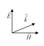
Anyway, for the higher multipoles, we are interested in spherical (but not spherically symmetric!) outgoing wave fronts.  In the far radiation zone, we will have waves which look locally a lot like the familiar plane waves. 

It does not follow from this that the $\overrightarrow{E},\overrightarrow{H}$ fields have zero components in the direction of propagation$—$it's just that these components get smaller and smaller (factor $\sim 1/r$ ) relative to the transverse components as the wave goes out. And, these components do play an essential role in radiation of angular momentum.

To learn more about possible field configurations, we need to solve Maxwell's equations in spherical polar coordinates.

Scalar Wave Equation

As a warm up exercise (which turns out to be very relevant) we begin with the spherical wave equation for a scalar field $\psi \left(x,y,z,t\right)$ before going on to the more difficult vector equations for the electric and magnetic fields. So we'll translate

${\nabla }^2\psi \left(x,y,z,t\right)-\frac{1}{c^2}\frac{{\partial }^2\psi \left(x,y,z,t\right)}{\partial t^2}=0$ 

into spherical polar coordinates.

Taking as usual time-dependence $e^{-i\omega t},$

$\psi \left(x,y,z,t\right)=\psi \left(x,y,z\right)e^{-i\omega t},$ 

 the spatial wave equation is

$\left({\nabla }^2+k^2\right)\psi \left(x,y,z\right)=0,k=\omega /c.$ 

This, of course, is identically the equation we solved for waveguides, but now we are going to use $r,\theta ,\varphi$ coordinates. 

However, it should still look familiar: ${\nabla }^2$ in spherical polars is exactly the equation for the hydrogen atom problem in elementary quantum mechanics, solved by separation of variables, and the same trick works here: the standard spherical harmonics expansion

$\psi \left(x,y,z\right)={\displaystyle \sum _{\ell ,m}{f}_{\ell m}\left(r\right)Y_{\ell m}\left(\theta ,\varphi \right)}$ 

where (to remind you)  $Y_{\ell m}\left(\theta ,\varphi \right)=\sqrt{\frac{2\ell +1}{4\pi }\cdot \frac{\left(\ell -m\right)!}{\left(\ell +m\right)!}}{P}_{\ell }^m\left(\cos \theta \right)e^{im\varphi }.$ 

Radial Wave Equation: Spherical Bessel Functions

The radial function satisfies (independent of $m$ )

$\left[\frac{d^2}{d{r}^2}+\frac{2}{r}\frac{d}{dr}+k^2-\frac{\ell \left(\ell +1\right)}{r^2}\right]f_{\ell }\left(r\right)=0.$ 

 At this point, Jackson makes the substitution $f_{\ell }\left(r\right)=u_{\ell }\left(r\right)/\sqrt{r},$ to find that $u_{\ell }\left(r\right)$ satisfies Bessel's equation for a half integer value $\nu =\ell +\frac{1}{2}:$ 

$\left[\frac{d^2}{d{r}^2}+\frac{1}{r}\frac{d}{dr}+k^2-\frac{{\left(\ell +\frac{1}{2}\right)}^2}{r^2}\right]u_{\ell }\left(r\right)=0.$ 

So $u_{\ell }\left(r\right)$ satisfies Bessel's equation$—$except that $\ell$ is replaced by $\ell +\frac{1}{2}.$ Recall that the usual Bessel's equation arises from the ${\nabla }^2$ operator expressed in cylindrical coordinates, we've just derived the same equation but with $\ell \to \ell +\frac{1}{2}$ from ${\nabla }^2$ in spherical coordinates. The solutions to this new version are called, not surprisingly, the spherical Bessel (Neumann, Hankel) functions, written using lower case $j_{\ell }\left(r\right)$, etc., and can be derived from the ordinary (cylindrical) Bessel functions (expressed in series form) as follows:

$\begin{array}{l}{j}_{\ell }\left(r\right)=\sqrt{\pi /2r}{J}_{\ell +\frac{1}{2}}\left(r\right),\\ n_{\ell }\left(r\right)=\sqrt{\pi /2r}{N}_{\ell +\frac{1}{2}}\left(r\right),\\ h_{\ell }{}^{(1,2)}\left(r\right)=\sqrt{\pi /2r}\left[J_{\ell +\frac{1}{2}}\left(r\right)\pm i{N}_{\ell +\frac{1}{2}}\left(r\right)\right].\end{array}$ 

 That is, we can find $j_{\ell }\left(r\right)$ from the infinite series expansions of the ordinary Bessel functions, for example

$J_{\nu }\left(r\right)={\left(\frac{r}{2}\right)}^{\nu }{\displaystyle \sum _{j=0}^{\infty }\frac{{\left(-1\right)}^j}{j!\Gamma \left(j+\nu +1\right)}{\left(\frac{r}{2}\right)}^{2j}}$ 

and using $\Gamma \left(\frac{1}{2}\right)=\sqrt{\pi },\Gamma \left(\frac{3}{2}\right)=\frac{1}{2}\sqrt{\pi },\Gamma \left(n\right)=\left(n-1\right)\Gamma \left(n-1\right)$ we find:

$j_0\left(r\right)=\frac{\sin r}{r},j_1\left(r\right)=\frac{\sin r}{r^2}-\frac{\cos r}{r},\dots$ 

Surprise: they turn out to be a lot simpler than the original Bessel functions!

The spherical Bessel functions are finite polynomials in $1/r$ with coefficients $\sin r,\cos r.$ The only justification for deriving them as we just did is to show why they're called Bessel functions.  It's far simpler to derive them by writing $f_{\ell }\left(r\right)=u_{\ell }\left(r\right)/r$ in the original differential equation as in every introductory quantum mechanics text!  In particular, I give a full treatment (based on Landau's presentation) in my graduate quantum mechanics notes here.

Asymptotically for large $r,$ 

$\begin{array}{l}{j}_{\ell }\left(r\right)\to \frac{1}{r}\sin \left(r-\frac{\ell \pi }{2}\right),\\ n_{\ell }\left(r\right)\to -\frac{1}{r}\cos \left(r-\frac{\ell \pi }{2}\right),\\ h_{\ell }{}^{\left(1\right)}\left(r\right)\to \frac{{\left(-i\right)}^{\ell +1}{e}^{ir}}{r}.\end{array}$ 

That is, the spherical Hankel function $h_{\ell }{}^{\left(1\right)}\left(r\right)$ is the function corresponding to outgoing waves.  This is what we're interested in here, so we look for solutions of the form ${\displaystyle \sum _{\ell ,m}{A}_{\ell m}\left(kr\right)Y_{\ell m}\left(\theta ,\varphi \right)}.$  The $Y_{\ell m}$ (given explicitly near the beginning of this section) are the familiar angular eigenstates of the angular momentum operator $\overrightarrow{L}=\left(1/i\right)\left(\overrightarrow{r}\times \overrightarrow{\nabla }\right)$ familiar from quantum mechanics (of course, without the $\hslash$ )  essentially the gradient operator on the spherical surface, and of course $\overrightarrow{r}\cdot \overrightarrow{L}=0.$ 

That is,

$\begin{array}{c}{L}^2{Y}_{\ell m}=\ell \left(\ell +1\right)Y_{\ell m}\\ L_{+}{Y}_{\ell m}=\sqrt{\left(\ell -m\right)\left(\ell +m+1\right)}{Y}_{\ell m+1},\\ L_{-}{Y}_{\ell m}=\sqrt{\left(\ell +m\right)\left(\ell -m+1\right)}{Y}_{\ell m-1},\\ L_z{Y}_{\ell m}=m{Y}_{\ell m}.\end{array}$ 

Also, $\overrightarrow{L}\times \overrightarrow{L}=i\overrightarrow{L}.$ 

Multipole Formalism

From Maxwell's equations in empty space (with time dependence $e^{-i\omega t},\omega =ck$ ),

$\begin{array}{c}\overrightarrow{\nabla }\times \overrightarrow{E}=ik{Z}_0\overrightarrow{H},\overrightarrow{\nabla }\times \overrightarrow{H}=-ik\overrightarrow{E}/Z_0\\ \overrightarrow{\nabla }\cdot \overrightarrow{E}=0,\overrightarrow{\nabla }\cdot \overrightarrow{H}=0\end{array}$

it follows that

$\left({\nabla }^2+k^2\right)\overrightarrow{E}=0,\overrightarrow{\nabla }\cdot \overrightarrow{E}=0,$ 

and the same equations hold  for $\overrightarrow{H}.$ These equations can be solved in standard fashion for the three Cartesian $\left(x,y,z\right)$ coordinates, but we're interested in spherical outgoing waves, and there is no trivial separation of these vector equations in spherical coordinates $\left(r,\theta ,\varphi \right).$  So how do we proceed?

Jackson uses a clever solution by Bouwkamp and Casimir (1954): they solved the equations for the scalar quantities $\overrightarrow{r}\cdot \overrightarrow{E},\overrightarrow{r}\cdot \overrightarrow{H}.$ This copies the standard approach to waves in waveguides, where the approach is to first solve for the field component in the direction of propagation, $E_z$ or $H_z.$

In this spherical case,

${\nabla }^2\left(\overrightarrow{r}\cdot \overrightarrow{E}\right)=\overrightarrow{r}\cdot {\nabla }^2\overrightarrow{E}+2\overrightarrow{\nabla }\cdot \overrightarrow{E},$ 

and similarly for $\overrightarrow{H},$ so since $\overrightarrow{\nabla }\cdot \overrightarrow{E}=0,\overrightarrow{\nabla }\cdot \overrightarrow{H}=0$, and ${\nabla }^2\overrightarrow{E}=-k^2\overrightarrow{E},$  

$\left({\nabla }^2+k^2\right)\left(\overrightarrow{r}\cdot \overrightarrow{E}\right)=0,\left({\nabla }^2+k^2\right)\left(\overrightarrow{r}\cdot \overrightarrow{H}\right)=0.$ 

So $\overrightarrow{r}\cdot \overrightarrow{E}$ is a solution to the wave equation!   (As is $\overrightarrow{r}\cdot \overrightarrow{H}.$ )

The general outgoing solution is a series in spherical harmonics with accompanying Hankel functions,

$\psi \left(\overrightarrow{r}\right)={\displaystyle \sum _{\ell ,m}\left[A_{\ell m}^{\left(1\right)}{h}_{\ell }^{\left(1\right)}\left(kr\right)+A_{\ell m}^{\left(2\right)}{h}_{\ell }^{\left(2\right)}\left(kr\right)\right]Y_{\ell m}\left(\theta ,\varphi \right)}.$ 

To see how this works, we'll choose a particular multipole. 

Magnetic (and Electric) Multipole Fields

Following Jackson, we define a magnetic multipole field of order $\left(\ell ,m\right)$ by the conditions

$\begin{array}{c}\overrightarrow{r}\cdot {\overrightarrow{H}}_{\ell m}^{\left(M\right)}=\frac{\ell \left(\ell +1\right)}{k}{g}_{\ell }\left(kr\right)Y_{\ell m}\left(\theta ,\varphi \right),\\ \overrightarrow{r}\cdot {\overrightarrow{E}}_{\ell m}^{\left(M\right)}=0,\end{array}$ 

(so this is analogous to a waveguide TE mode) where $g_{\ell }\left(kr\right)=h_{\ell }^{\left(1\right)}\left(kr\right)$ for outgoing waves. We know this is a solution of the wave equation, and we can visualize the component of magnetic field that points perpendicularly outwards from a spherical surface having angular pattern $Y_{\ell m}\left(\theta ,\varphi \right)$ like a standing wave on a spherical balloon (and for bigger spherical surfaces, going down in magnitude as the inverse radius).

The electric field is only tangential, but it has the same angular pattern:  from Maxwell's equations,

$Z_{0}k\overrightarrow{r}\cdot \overrightarrow{H}=-i\overrightarrow{r}\cdot \left(\overrightarrow{\nabla }\times \overrightarrow{E}\right)=-i\left(\overrightarrow{r}\times \overrightarrow{\nabla }\right)\cdot \overrightarrow{E}=\overrightarrow{L}\cdot \overrightarrow{E}.$ 

Therefore (with $\left(M\right)$ denoting that this is a magnetic multipole)

$\overrightarrow{L}\cdot {\overrightarrow{E}}_{\ell m}^{\left(M\right)}\propto \overrightarrow{r}\cdot {\overrightarrow{H}}_{\ell m}^{\left(M\right)}\propto Y_{\ell m}\left(\theta ,\varphi \right).$ 

But if we expand this $\overrightarrow{E}$ in spherical harmonics, the operator $\overrightarrow{L}$ will generate adjacent ones,

so this can't be correct, unless $\overrightarrow{E}\left(\theta ,\varphi \right)$ is an eigenstate of $\overrightarrow{L}$:

$\begin{array}{l}{\overrightarrow{E}}_{\ell m}^{\left(M\right)}=Z_0{g}_{\ell }\left(kr\right)\overrightarrow{L}{Y}_{\ell m}\left(\theta ,\varphi \right),\\ H_{\ell m}^{\left(M\right)}=-\left(i/k{Z}_0\right)\overrightarrow{\nabla }\times {\overrightarrow{E}}_{\ell m}^{\left(M\right)},\end{array}$ 

in which case $\overrightarrow{L}\cdot {\overrightarrow{E}}_{\ell m}^{\left(M\right)}\propto L^2{Y}_{\ell m}\left(\theta ,\varphi \right).$ 

To see the magnetic field pattern, notice that

$\overrightarrow{r}\cdot \overrightarrow{H}\propto \overrightarrow{r}\cdot \overrightarrow{\nabla }\times \overrightarrow{E}\propto \overrightarrow{r}\cdot \overrightarrow{\nabla }\times \overrightarrow{L}{Y}_{\ell m}=\left(\overrightarrow{r}\times \overrightarrow{\nabla }\right)\cdot \overrightarrow{L}{Y}_{\ell m}=L^2{Y}_{\ell m}=\ell \left(\ell +1\right)Y_{\ell m}.$ 

The electric multipole fields are defined in the same way, with the fields swapped:

  

$\begin{array}{l}\overrightarrow{r}\cdot {\overrightarrow{E}}_{\ell m}^{\left(E\right)}=-Z_0\left(\frac{\ell \left(\ell +1\right)}{k}\right)f_{\ell }\left(kr\right)Y_{\ell m}\left(\theta ,\varphi \right),\\ \overrightarrow{r}\cdot {\overrightarrow{H}}_{\ell m}^{\left(E\right)}=0.\end{array}$ 

The electric multipole fields are

$\begin{array}{l}{\overrightarrow{H}}_{\ell m}^{\left(E\right)}=f_{\ell }\left(kr\right)\overrightarrow{L}{Y}_{\ell m}\left(\theta ,\varphi \right),\\ {\overrightarrow{E}}_{\ell m}^{\left(E\right)}=\frac{i{Z}_0}{k}\overrightarrow{\nabla }\times {\overrightarrow{H}}_{\ell m}^{\left(E\right)}.\end{array}$ 

Vector Spherical Harmonics

It's useful to introduce a bit more notation, the so-called vector spherical harmonics:

${\overrightarrow{X}}_{\ell m}\left(\theta ,\varphi \right)=\frac{1}{\sqrt{\ell \left(\ell +1\right)}}\overrightarrow{L}{Y}_{\ell m}\left(\theta ,\varphi \right).$ 

These have simple orthogonality properties:

$\begin{array}{l}{\displaystyle \int {\overrightarrow{X}}^{\ast }{}_{{\ell }^{\prime }{m}^{\prime }}}\cdot {\overrightarrow{X}}_{\ell m}={\delta }_{\ell {\ell }^{\prime }}{\delta }_{m{m}^{\prime }},\\ {\displaystyle \int {\overrightarrow{X}}^{\ast }{}_{{\ell }^{\prime }{m}^{\prime }}}\cdot \left(\overrightarrow{r}\times {\overrightarrow{X}}_{\ell m}\right)d\Omega =0.\end{array}$ 

At this point, Jackson states (but does not prove) that these two types of waves form a complete set of vector solutions to Maxwell’ equations in the source-free region. That is, the general solution is

$\begin{array}{l}\overrightarrow{H}={\displaystyle \sum _{\ell m}\left[a_E\left(\ell ,m\right)f_{\ell }\left(kr\right){\overrightarrow{X}}_{\ell m}-\frac{i}{k}{a}_M\left(\ell ,m\right)\overrightarrow{\nabla }\times g_{\ell }\left(kr\right){\overrightarrow{X}}_{\ell m}\right]}\\ \overrightarrow{E}=Z_0{\displaystyle \sum _{\ell m}\left[\frac{i}{k}{a}_E\left(\ell ,m\right)\overrightarrow{\nabla }\times f_{\ell }\left(kr\right){\overrightarrow{X}}_{\ell m}+a_M\left(\ell ,m\right)g_{\ell }\left(kr\right){\overrightarrow{X}}_{\ell m}\right]}\end{array}$

where $a_E\left(\ell ,m\right),a_M\left(\ell ,m\right)$ are the amplitudes of the electric and magnetic multipole fields. The radial functions are Hankel functions, exactly as in the scalar case above, $\psi \left(\overrightarrow{r}\right)={\displaystyle \sum _{\ell ,m}\left[A_{\ell m}^{\left(1\right)}{h}_{\ell }^{\left(1\right)}\left(kr\right)+A_{\ell m}^{\left(2\right)}{h}_{\ell }^{\left(2\right)}\left(kr\right)\right]Y_{\ell m}\left(\theta ,\varphi \right)}.$

The coefficients can be determined if $\overrightarrow{r}\cdot \overrightarrow{H}$ and $\overrightarrow{r}\cdot \overrightarrow{E}$ are known,

$a_M\left(\ell ,m\right)=\frac{k}{\sqrt{\ell \left(\ell +1\right)}}{\displaystyle \int \begin{array}{l}{Y}_{\ell m}^{*}\overrightarrow{r}\cdot \overrightarrow{H}d\Omega \\ \end{array}}$

$\begin{array}{l}{a}_M\left(\ell ,m\right)g_{\ell }\left(kr\right)=\frac{k}{\sqrt{\ell \left(\ell +1\right)}}{\displaystyle \int Y_{\ell m}^{*}\overrightarrow{r}\cdot \overrightarrow{H}d\Omega },\\ Z_0{a}_E\left(\ell ,m\right)f_{\ell }\left(kr\right)=-\frac{k}{\sqrt{\ell \left(\ell +1\right)}}{\displaystyle \int Y_{\ell m}^{*}\overrightarrow{r}\cdot \overrightarrow{E}d\Omega }.\end{array}$

Using the Result

In the rest of Chapter 9, Jackson uses these expressions to find the energy and angular momentum of multipole radiation, for atoms, nuclei and a center-fed linear antenna. We will not cover this material here.  

previous  index  next