71.  Motion of a Spin One-Half in a Slowly-Varying Magnetic Field:
The Key to Measuring the Muon Moment (g $–$ 2)

Jackson 11.11,  plus discussion of g-2.

Michael Fowler, UVa

Introduction

It turns out that when an electron or a muon moves through a magnetic field, the spin direction closely follows the velocity direction. The small difference in rotation rate, of order one part in a thousand, can be measured extremely accurately$—$so well that contributions from strong interactions (as explained below) can be detected and measured. That is to say, this experiment, with no hadrons in sight, can be used to test quantum chromodynamics calculations, and thereby improve our (inadequate) understanding of strong interactions. The experiment is judged sufficiently important that the recent (2022) annual dollar cost runs to nine figures.

Nonrelativistic Limit: the g-factor

The plan is to track how the direction of the spin vector changes as an electron (or muon) moves along a given path through a slowly varying, time independent magnetic field. (The spin, of course, has an accompanying magnetic moment.)

First, the unit for measuring particle magnetic moments is the Bohr magneton, the magnetic moment of the current loop corresponding to an electron in the lowest Bohr model orbit, the $\mathcal{l}=1$ orbit having angular momentum $\hslash .$ (We’re just explaining the origin of the term$—$we know now of course that Bohr’s model was flawed, even though it correctly predicted energy differences: the lowest actual hydrogen atom state has $\mathcal{l}=0.$ )  For this simple “classical” Bohr picture, thinking of the electron as a particle of mass $m$ and charge $e$ moving in a circle of radius $r$ at speed $v,$ the angular momentum is $mvr=\hslash ,$ and the electric current is $ev/2\pi r$ so this “current loop” has magnetic moment current x area (see lecture 31) $$

$${\mu }_{\text{B}}=IA=ev/\left(2\pi r\right)\pi r^2=\frac{1}{2}evr=e\hslash /2m.$$

Experimentally, the electron has an intrinsic angular momentum (spin) $s_z=\pm \frac{1}{2}\hslash ,$ and accompanying magnetic moment (SI, gaussian has a c in the denominator)

$$\overrightarrow{\mu }=\left(ge/2m\right)\overrightarrow{s},g\cong \mathrm{2.002...}$$

Note that if the electron is modeled as a classical spinning charge distribution, that would give $g=1,$ just as for the Bohr orbit above. On the other hand, Dirac’s linear, relativistically-invariant, equation predicts $g=2,$ very close to that observed, an impressive feat. The further 0.002… correction is mainly a quantum electrodynamic effect, and theoretical predictions based on that theory give close agreement with experiment, as discussed in detail below.

Electron Spin Precession, Classical and Quantum

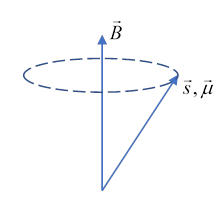
We’ll consider first an electron at the origin in a constant magnetic field $\overrightarrow{B}=B\widehat{\overrightarrow{z}}.$ It has a magnetic energy $U=-\overrightarrow{\mu }\cdot \overrightarrow{B},$ and the field exerts a couple $\overrightarrow{\mu }\times \overrightarrow{B}$ on the particle, causing precession around the magnetic field direction:

$$d\overrightarrow{s}/dt=\overrightarrow{\mu }\times \overrightarrow{B}=\left(ge/2m\right)\overrightarrow{s}\times \overrightarrow{B},$$

with a frequency $\omega =geB/2m.$ 

Exercise:  Check this by drawing $d\overrightarrow{s}$ on the diagram.

To reassure ourselves that this classical result is also good for the electron quantum spin one-half (following Landau) we write the Hamiltonian for the spin one-half magnetic field interaction in terms of the Pauli matrices,

$$\widehat{H}={\widehat{H}}_0-\mu \overrightarrow{\sigma }\cdot \overrightarrow{B},\overrightarrow{s}=\frac{1}{2}\hslash \overrightarrow{\sigma },$$

with ${\widehat{H}}_0$ the spin-independent terms,  $\mu =ge\hslash /4m_e$ (SI units), and $\overrightarrow{B}$ the magnetic field at the particle position.

We’ll for the present take $g=2,$ and address the (important!) difference later.

The operator equation of motion is, writing spin $\overrightarrow{s}=\frac{1}{2}\hslash \overrightarrow{\sigma },$ (Landau, p 152)

$$\dot{\overrightarrow{s}}=\frac{i}{2\hslash }\left(\widehat{H}\overrightarrow{\sigma }-\overrightarrow{\sigma }\widehat{H}\right),$$

 from which

$$\begin{array}{c}{\dot{s}}_i=-\frac{i\mu }{2\hslash }{B}_k\left({\sigma }_k{\sigma }_i-{\sigma }_i{\sigma }_k\right)\\ =-\frac{\mu }{\hslash }{\epsilon }_{ikl}{B}_k{\sigma }_l\\ =\frac{2\mu }{\hslash }{\left(\overrightarrow{s}\times \overrightarrow{B}\right)}_i=\frac{ge}{2m}{\left(\overrightarrow{s}\times \overrightarrow{B}\right)}_i\end{array}$$

This is in fact identical to the classical equation!

Bottom line:

The spin precesses about the field direction with angular velocity $-geB/2m.$

This is Jackson 11.155, in SI units, although his is for the rest frame (and his $t^{\prime }$ is time in that frame, in preparation for going to the relativistic case).

For an electron moving through a slowly varying magnetic field, this will give the current spin precession rate.

But the velocity vector is also “precessing” (remember its magnitude is constant if there is no electric field), and (nonrelativistically), it satisfies

$$m\frac{d\overrightarrow{v}}{dt}=e\overrightarrow{v}\times \overrightarrow{B}.$$

That is, the velocity vector rotates about $\overrightarrow{B}$ at angular velocity $-eB/m.$

Comparing the two: IF $g=2,\mu =e\hslash /2m,$

the spin direction and the velocity direction precess at the same rate

meaning the spin polarization vector is at a constant angle to the direction of motion.

But $g\ne 2,$ and spin observation is the key to finding the small quantity $g-2:$ the angle between spin direction and velocity direction will slowly change, and that rate of change can be measured experimentally.

Relativistic Generalization

Remarkably, it turns out that this constant angle between spin and momentum (for motion in a magnetic field) is still valid relativistically, provided $\mu =e\hslash /2m,$ meaning $g=2.$ 

To prove this, though, we need to write the spin equation of motion in a relativistically invariant way. Clearly we must go to proper time $\tau ,$ and we must promote the spin $\overrightarrow{s}$ to a four-vector, by constructing the four-vector that reduces to the spin three-vector in the particle rest frame.

(Notation warning: We’ll follow Jackson’s notation, but it needs care$—$it’s font case dependent, lower case is used for spin in the rest frame, upper case for lab frame.

Landau avoids this by writing the four-spin as $a^{\alpha },$ ( $a$ for axial, I think, because, like angular momentum, it’s even under reflection $\overrightarrow{x}\to -\overrightarrow{x}.$ ) However, in doing this same problem Garg uses $a^{\alpha }$ for the four-acceleration$—$the standard notation. Zangwill doesn’t cover any of this.

Generalizing the Spin to Four Dimensions

Following Jackson, section 11.11A, we define a four-vector $S^{\alpha }=\left(S^0,\overrightarrow{S}\right)$ in inertial frame $K$ by requiring that in the particle’s rest frame $K^{\prime }$  it is $\left(0,{\overrightarrow{s}}^{\prime }\right).$ That is, in the particle rest frame the spin time component $S^0{}^{\prime }=0.$ 

The four-spin components $S^{\alpha }$ in other frames then follow from the usual vector Lorentz transformations.

Note that since the particle’s four-velocity in the rest frame $U^{\alpha }=\left(c,0,0,0\right)$, and the inner product $U^{\alpha }{S}_{\alpha }$ is Lorentz invariant,  $U^{\alpha }{S}_{\alpha }=0$ in all frames. 

*Four-Spin in Different Frames

This section (which follow Jackson) can be skipped at first reading.

In preparation for looking at the spin in different frames, Jackson next rewrites his earlier transformation equations (11.22) for an arbitrary four-vector $A^{\alpha }$ (identical of course to the equations for the position coordinate vector).  He uses the standard notation of denoting with $A_{\parallel },{\overrightarrow{A}}_{\perp }$ the three-vector components parallel and perpendicular to the relative velocity $\overrightarrow{\beta }c$ of the two frames. The equations can then be written (his 11.22)

$$\begin{array}{c}{A^{\prime }}_0=\gamma \left(A_0-\beta A_{\parallel }\right),\\ {A^{\prime }}_{\parallel }=\gamma \left(A_{\parallel }-\beta A_0\right),\\ {\overrightarrow{A^{\prime }}}_{\perp }={\overrightarrow{A}}_{\perp }.\end{array}$$

Exercise: Check this is correct for the relative velocity along the $z$ -axis.

Translating this to the spin components in the two frames, in the spin rest-frame $K^{\prime }$ the four-vector

$$\left({S^{\prime }}_0,{\overrightarrow{s}}^{\prime }\right)=\left(0,{\overrightarrow{s}}^{\prime }\right)\equiv \left({A^{\prime }}_0,{\overrightarrow{A}}^{\prime }\right),$$

so the first (time component) spin equation (transcribing from the ${A^{\prime }}_0$ equation above) is

$$S_0{}^{\prime }=\gamma \left(S_0-\overrightarrow{\beta }\cdot \overrightarrow{S}\right),$$

and since $S_0{}^{\prime }=0$ (by definition),

$$S_0=\overrightarrow{\beta }\cdot \overrightarrow{S}.$$

Putting this in the second equation gives

$${\overrightarrow{s}}_{\parallel }{}^{\prime }=\gamma \left({\overrightarrow{S}}_{\parallel }-\beta S_0\right),$$

$${\overrightarrow{s}}^{\prime }\cdot \overrightarrow{\beta }=\gamma \left(\overrightarrow{S}\cdot \overrightarrow{\beta }-{\beta }^2\left(\overrightarrow{S}\cdot \overrightarrow{\beta }\right)\right).$$

(Notation: Unlike Jackson, we’ve put a prime on ${\overrightarrow{s}}^{\prime }$ to remind ourselves it’s in the spin rest frame $K^{\prime }.$ )

In fact, from the third equation, the components of ${\overrightarrow{s}}^{\prime },\overrightarrow{S}$ are identical except in the $\overrightarrow{\beta }$ (longitudinal) direction, so it follows from the above that (Jackson 11.158)

$${\overrightarrow{s}}^{\prime }=\overrightarrow{S}-\left(\frac{\gamma }{\gamma +1}\right)\left(\overrightarrow{\beta }\cdot \overrightarrow{S}\right)\overrightarrow{\beta }.$$

Exercise: Prove it.

The inverse expressions are (all from Jackson)

$$\begin{array}{c}\overrightarrow{S}={\overrightarrow{s}}^{\prime }+\frac{{\gamma }^2}{\gamma +1}\left(\overrightarrow{\beta }\cdot {\overrightarrow{s}}^{\prime }\right)\overrightarrow{\beta },\\ S_0=\gamma \overrightarrow{\beta }\cdot {\overrightarrow{s}}^{\prime }.\end{array}$$

Relativistic Spin Precession: the BMT Equation

We’re now ready to construct a Lorentz invariant equation for the (proper) time development of the four-spin, $d{S}^{\alpha }/d\tau .$ Here we’ll follow Landau’s (only slightly different) presentation (page 153, QED Vol 4, 2^nd ed).  The expression must be linear and homogeneous in $F^{\alpha \beta }$ and $S^{\alpha },$ and the only other variable is $U^{\alpha }.$ (Jackson further includes $d{U}^{\alpha }/d\tau ,$ but that is $\left(e/m\right)F^{\alpha \beta }{U}_{\beta }$, so adds nothing new).

With these requirements, the equation must be

$$\frac{d{S}^{\alpha }}{d\tau }=A{F}^{\alpha \beta }{S}_{\beta }+B{U}^{\alpha }{F}^{\beta \gamma }{U}_{\beta }{S}_{\gamma },$$

with $A,B$ constant coefficients. Landau remarks that with $U_{\alpha }{S}^{\alpha }=0,$ and $F^{\alpha \beta }$ antisymmetric so $F^{\alpha \beta }{U}_{\alpha }{U}_{\beta }=0,$ it’s not difficult to check that there can be no other linear homogeneous terms (try writing one).

In the nonrelativistic limit, from our definition of the four-dimensional spin (that it’s $\left(0,{\overrightarrow{s}}^{\prime }\right)$ in the rest frame) the left-hand side will only have spatial components, and in this limit the second term on the right hand side won’t contribute, since $U^{\alpha }\to \left(c,0,0,0\right),$ (and $U_{\alpha }\to \left(-c,0,0,0\right)$ with our metric -+++).

We already know the equation must become

$${\dot{s}}_i=\frac{2\mu }{\hslash }{\left(\overrightarrow{s}\times \overrightarrow{B}\right)}_i,$$

so that fixes the first unknown constant $A:$

$$A=\frac{2\mu }{\hslash }=\frac{ge}{2m}.$$

The remaining task is to find the constant $B.$

The trick is to differentiate $U^{\alpha }{S}_{\alpha }=0$:

$$\frac{d}{d\tau }\left(U_{\alpha }{S}^{\alpha }\right)=S^{\alpha }\frac{d{U}_{\alpha }}{d\tau }+U_{\alpha }\frac{d{S}^{\alpha }}{d\tau }=0$$

and then insert the equation of motion

$$m\frac{d{U}^{\alpha }}{d\tau }=e{F}^{\alpha \beta }{U}_{\beta }$$

to find

$$U_{\alpha }\frac{d{S}^{\alpha }}{d\tau }=-S_{\alpha }\frac{d{U}^{\alpha }}{d\tau }=-S_{\alpha }\frac{e}{m}{F}^{\alpha \beta }{U}_{\beta }=\frac{e}{m}{F}^{\alpha \beta }{U}_{\alpha }{S}_{\beta }$$

where we switch up-down index pairs to down-up, and used the antisymmetry of $F^{\alpha \beta }$ in the last step.

Now, recalling $d{S}^{\alpha }/d\tau =A{F}^{\alpha \beta }{S}_{\beta }+B{U}^{\alpha }{F}^{\beta \gamma }{U}_{\beta }{S}_{\gamma },$ and multiplying both sides by $U_{\alpha },$ remembering that $U^{\alpha }{U}_{\alpha }=-c^2$

$$\frac{e}{m}{F}^{\alpha \beta }{U}_{\alpha }{S}_{\beta }=A{F}^{\alpha \beta }{U}_{\alpha }{S}_{\beta }-c^{2}B{F}^{\beta \gamma }{U}_{\beta }{S}_{\gamma }.$$

Notice that all indices are dummies, so all terms have identical structure, and recalling $A=ge/2m,$ we have

$$\frac{e}{m}=\frac{ge}{2m}-B{c}^2,$$

and

$$B=\frac{e}{2m{c}^2}\left(g-2\right).$$

Now that we’ve found $A$ and $B,$ the relativistic spin precession equation

$$\frac{d{S}^{\alpha }}{d\tau }=A{F}^{\alpha \beta }{S}_{\beta }+B{U}^{\alpha }{F}^{\beta \gamma }{U}_{\beta }{S}_{\gamma }$$

can be written

$$\frac{d{S}^{\alpha }}{d\tau }=\frac{ge}{2m}{F}^{\alpha \beta }{S}_{\beta }+\frac{e}{2m{c}^2}\left(g-2\right)U^{\alpha }{F}^{\beta \gamma }{U}_{\beta }{S}_{\gamma }.$$

(Jackson 11.164, he has an extra c in the denominator because he’s using gaussian units here.)

Comparing this with the equation of motion

$$m\frac{d{U}^{\alpha }}{d\tau }=e{F}^{\alpha \beta }{U}_{\beta }$$

we see directly that for $g=2$ the four-vectors for spin and velocity precess together, generalizing the nonrelativistic result that for $g=2$ the angle between spin and velocity is constant. We can also see that for $g=\mathrm{2.002...}$ the angle will change only slowly, and the rate of change is a direct measure of $g-2.$ 

The spin precession equation above is called the BMT equation, found by Bargmann, Michel and Telegdi in 1959 (but previously found by Thomas in 1927 and Frenkel in 1926).

The rest of this lecture, an outline of the relevant particle physics, is optional.

*Theoretical Calculation of Electron and Muon Magnetic Moments

As mentioned at the beginning of the lecture, the first naïve ideas about these moments, based on the misconception that the electron spin $\overrightarrow{s}$ was equivalent to some classical rotating charge distribution, predicted that $\overrightarrow{\mu }=\left(ge/2m\right)\overrightarrow{s}$ with (wrongly) $g=1.$ The first relativistic wave equation for a spin one-half particle was Dirac’s in 1928.  It impressively gave $g=2,$ only off by a part in a thousand or so$—$but nevertheless off.

The big breakthrough came in 1949 with Schwinger’s quantum electrodynamic calculation that to leading order in perturbation theory

$$\frac{g}{2}=1+\frac{\alpha }{2\pi },$$

where the fine structure constant $\alpha \cong 1/137,$ so $g\cong \mathrm{2.00232.}$

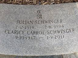
This result, with $g$ now correct to about a part in a million, gained Schwinger the Nobel prize, and is written on his gravestone.

In a later review paper, Schwinger attributed the achievement to “George Green and I” (as we mentioned earlier in the lecture on Green’s functions). 

However, this is not the end of the story. The experimental results are much more precise, challenging theorists to compute higher orders of perturbation theory.

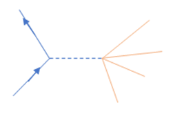
Just to give a taste of the quantum electrodynamics involved, in Feynman diagram language the electron (or muon) is represented as a solid line, the electromagnetic field is a photon$—$but off its mass shell, meaning non-propagating. (For example, a static field is built of such photons).  The interaction is called a “vertex” (see figure).

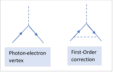
 The first order correction, the $\alpha /2\pi$ calculated by Schwinger, in this diagram language corresponds to the emission and subsequent reabsorption of a virtual photon bridging the magnetic interaction (as in the diagram on the right).

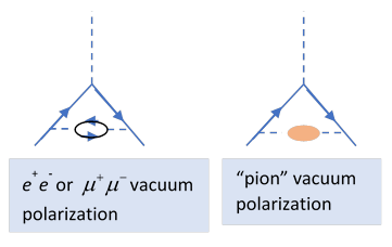
Many higher order quantum electrodynamic diagrams can be drawn. An important one turns out to be that of the “bridging” photon line (which is of course an electromagnetic field) polarizing the vacuum, creating virtual electron-positron pairs, or muon-antimuon pairs, as shown on the left here.  

Including all the second-order QED diagrams (which means a lot of calculation, see Landau) gives for the magnetic moment of the electron

$${\mu }_e={\frac{e\hslash }{2m}}_e\left(1+\frac{\alpha }{2\pi }-0.328\frac{{\alpha }^2}{{\pi }^2}\right).$$

Noting that the electron mass does not appear inside the bracket, one might conclude that the same second-order expression would work for the muon, just by changing the outside mass term. However, this is not quite right: the problem is the vacuum polarization loop. For the electron, this calculation includes the electron-positron loop, which is fine, because the muon-antimuon loop makes a much smaller contribution.  However, in calculating the muon magnetic moment, this same expression includes the muon-antimuon loop (which contributes around 2% of the total), but does not include the electron-positron loop, which is more important since the lighter virtual particles are more easily excited.  

Now including the electron-positron polarization loop, the muon magnetic moment to second order is

$${\mu }_{\mu }=\frac{e\hslash }{2m_{\mu }c}\left(1+\frac{\alpha }{2\pi }+0.76\frac{{\alpha }^2}{{\pi }^2}\right).$$

These results are often presented in terms of the parameter

$$a=\frac{g-2}{2}.$$

The original calculation gives $a_{\mu }=0.00116141,$ the second-order term shown above brings this to $a_{\mu }=\mathrm{0.00116551.}$ (Not great notation, but standard: watch out for $a,\alpha$!)

The muon-antimuon loop contributes of order $\mathrm{0.0000001.}$ As we shall see, the experiment delivers greater accuracy than the numbers we have given so far$—$the current experimental result is $a_{\mu }=\mathrm{0.001165920.}$ But the higher order graphs in quantum electrodynamics (meaning interactions of photons, electrons, positrons, muons and antimuons) solved in perturbation theory are multiplied by powers of the fine structure constant, $1/137,$ and are not big enough to reproduce the measured result.

Enter the Standard Model

What are we missing?  Well, we’ve ignored a lot of other particles. We found a significant contribution to the vacuum polarization term from the muon-antimuon loop, but the (charged) pion has a mass not much greater that the muon, so surely there has to be a pion-antipion loop too?  But it’s not that simple. The pion is strongly interacting, you can’t treat the strong interactions with perturbation theory, so the loop will be a strongly interacting mess, we represent it by a blob in the fourth diagram (as do others). However, this is what makes it interesting. We have a very exact result from experiment, so this is a good test of various theoretical attempt to analyze the strong interactions quantitatively. In particular, recent results using lattice gauge theory look good.

(Another approach we mention only for experts: the imaginary part of the polarization amplitude is given by all the hadronic blob components being on their mass shell, i.e. real, not virtual, particles. And, thanks to the magic of Feynman diagrams, this same graph represents an electron meeting a positron and annihilating into a photon which generates a spray of hadrons, as depicted here. This process occurs and these amplitudes have been measured. Then, by analytic continuation we can (with effort!) get to the hadronic contribution to the muon magnetic moment.)

This new insight into the murky world of strong interactions is a major reason the $g-2$ experiment is worth doing.

The Experiment

If a muon is injected into a uniform magnetic field, in a direction perpendicular to the field, it will follow a circular path. If the injected muon has its spin aligned with its direction of motion (“polarized”), then, from the discussion above, after a complete circle the velocity vector will have rotated through 360 degrees, for $g=2$ the spin would have done the same, but with $g-2$ of order 0.001, the spin will be at a small angle (about a third of a degree) to the direction of motion, and this deviation increases linearly with the number of orbits. When the muon decays (its lifetime is about 2 microseconds) it emits an electron in the direction its spin was pointing, so by detecting this electron the accumulated change of spin direction can be found, and thus $g-2$ measured.  

In the current experiment at Fermilab, polarized muons having energy about 3.1 GeV are injected into a storage ring of diameter fifty feet in a perpendicular uniform magnetic field of strength 1.45 Tesla. Since the muons are traveling essentially at the speed of light (one foot per nanosecond!) one circuit takes about 0.15 microseconds.

The muon mass is around $100\text{ MeV}/c^2,$ so the relativistic $\gamma \simeq 30.$ The muon lifetime is 2 microseconds in its rest frame, so the lab lifetime is around 60 milliseconds, in that time it would go around thousands of times, there will evidently be large total precession angles.

Further technical info (from Stefan Baessler): More precisely, the experiment is run at $\gamma =\mathrm{29.3,}$ referred to as the magic gamma, because it turns out that the effect of the motional magnetic field from the focussing electric quadrupoles on the precession vanishes at that value.

History of the Experiment

Measuring the muon magnetic moment to this accuracy is the modern equivalent of building a medieval cathedral. The experiment began in 1959, and will not end any time soon. Many thousands of highly skilled workers have spent years on it, and the cost runs to billions of dollars.

The first project was at CERN, and in the early sixties confirmed Schwinger’s result. The second stage began at Brookhaven Lab, on Long Island, in 1989, a factor of 20 more precise than the CERN experiment. This involved the muon storage ring mentioned above. Finally (possibly!) in 2013 the experiment was moved to Fermilab. Transporting the fifty-foot diameter ring proved challenging: it could not be disassembled. The simplest route from Long Island, NY, to Chicago for such a load turned out to include going by sea around Florida$—$the details can be found here.

previous  index  next <