previous  index  next 

6. Electrostatics I: Fields, Potentials, Energy

    Michael Fowler, UVa

Coulomb’s Law

In 1785, Coulomb in France measured the force of repulsion between small charged conducting spheres and concluded that it went as the inverse of the square of the distance between the spheres.

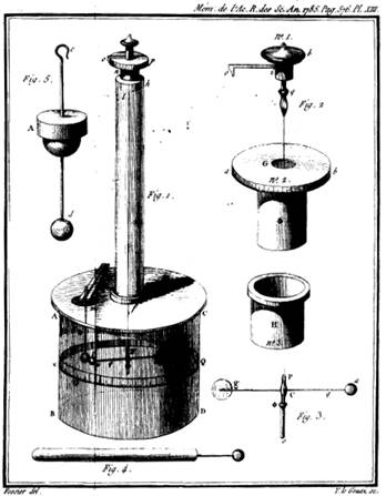
One of the spheres was at the end of a horizontal arm suspended by a wire (this is his original figure, see the little guy inside that bottom cylinder), the twist in the wire providing a measurable restoring force, proportional to angle turned through, as the other sphere approached, so the distance between spheres could be adjusted and the force measured.

Actually this inverse square law had been tested years earlier by Cavendish in England (1773), who concluded that the exponent was $2.00\pm 0.02$, so most likely exactly 2.

Cavendish used a quite different method: it can be shown (as we'll discuss later) that there is zero electric field inside a closed hollow charged conductor (easy to prove for a sphere), and this is only the case for an inverse square law of force.  So Cavendish just measured this field very accurately, and was able to determine the exponent to be 2 within about 1%.

But: Cavendish didn’t publish his result!  He wrote it up in notebooks, to be rediscovered by Maxwell and published long after Cavendish died. The notebooks are online here .

(Of course, we now know the exponent is 2 within a part in 10¹⁵ or so, so we won’t worry about it further.)  The inverse square law is good from a galaxy scale down to a subatomic scale, and therefore for any system considered in this course.

Furthermore, the linearity of the equations (fully confirmed by experiment for field strengths we will encounter) ensures that the total force on one charge in a system is the vector sum of the forces from all the other charged particles.

Faraday’s Picture of the Electric Field: Lines Under Tension, with Sideways Repulsion

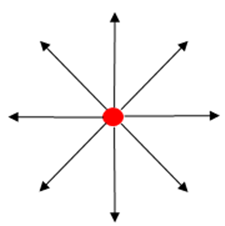
Perhaps the most profound concept in electrostatics, the electric field, was conceived by a mathematically illiterate but extremely talented experimentalist, Michael Faraday.  Faraday’s insights were later translated into equations by Maxwell, and so made available to a much wider audience. In fact, Faraday had a real understanding of the physics: his picture was that from a positive charge “lines of force” radiated outwards, just like fluid from a source, so naturally the density of these lines went down as the inverse square (in three dimensions), and furthermore these lines repelled each other sideways, giving an even spread from a single source, and at least a qualitative understanding of the field pattern from two separated positive charges. or a pair of opposite charges.

Exercise:  Try sketching lines of forces for two charges. The lines flow out from a positive, into a negative charge, like water moving from a source, then into a sink.  Draw the field lines for two equal and opposite charges some distance apart, then for two equal positive charges, then unequal positive and negative charges.

Maxwell was able to reduce these insights to precise mathematical formulation: these fields in space are real, they have spatial energy and stress density, analogous to that inside a stressed elastic solid.  We'll discuss this in much more detail later.

Definition of the Electric Field;  Field from a Distribution of Charges

The electric field strength $\overrightarrow{E}$ is defined in terms of the electric force $\overrightarrow{F}$ experienced by a very small (so it won't disturb the others) “test” charge $q$ placed in some environment where charges are present,

$\overrightarrow{F}=q\overrightarrow{E}$.

Coulomb’s law is that the force of repulsion experienced by a charge $q_1$ at ${\overrightarrow{r}}_1$ from a charge $q_2$ at ${\overrightarrow{r}}_2$ is (using the SI value for the overall constant):

$$\overrightarrow{F}=\frac{q_1{q}_2}{4\pi {\epsilon }_0}\cdot \frac{{\overrightarrow{r}}_1-{\overrightarrow{r}}_2}{{\left|{\overrightarrow{r}}_1-{\overrightarrow{r}}_2\right|}^3}.$$

 

Therefore, from our definition, the electric field from a single charge $q_1$ at ${\overrightarrow{r}}_1$ is:

$$\overrightarrow{E}\left(\overrightarrow{r}\right)=\frac{q_1}{4\pi {\epsilon }_0}\frac{\overrightarrow{r}-{\overrightarrow{r}}_1}{{\left|\overrightarrow{r}-{\overrightarrow{r}}_1\right|}^3}.$$ 

The electric field from a collection of charges is simply the linear sum, and generalizing to a continuous distribution,

$$\overrightarrow{E}\left(\overrightarrow{r}\right)=\frac{1}{4\pi {\epsilon }_0}{\displaystyle \int \rho \left({\overrightarrow{r}}^{\prime }\right)}\frac{\overrightarrow{r}-{\overrightarrow{r}}^{\prime }}{{\left|\overrightarrow{r}-{\overrightarrow{r}}^{\prime }\right|}^3}{d}^3{r}^{\prime }.$$ 

(This, of course, is an assertion that has to be established experimentally, and has been for all fields we'll encounter in this course. It only breaks down when the electromagnetic energy density is sufficient to generate virtual electron-positron pairs in measurable quantities.)

Maxwell’s First Equation: Gauss’s Law

Gauss’ law (in electrostatics) is that the “outflow” of electric field from a closed surface is equal to $q/{\epsilon }_0$, where $q$ is the charge in the volume the surface encloses, or

${\displaystyle \underset{S}{\int }\overrightarrow{E}\cdot d\overrightarrow{A}={\displaystyle \underset{V}{\int }\rho \left(\overrightarrow{r}\right)d^{3}r.}}$ 

As mentioned earlier, Faraday used the term electric flux (meaning flow) because he imagined some outgoing flow of “particles” emanating from a charge.  Why did he think in those terms?  Because the field strength from a single charge decreases as the inverse square with distance$—$that’s exactly how the flow field from a source of fluid goes down!  Imagine a steady source of (incompressible) fluid deep in a pool of the fluid, like the end of a hose, but arranged to send out fluid equally in all directions, say $q$ cubic meters per second.  In a steadily flowing situation, the flow rate across a spherical surface centered at the source, ${\displaystyle \int \rho \overrightarrow{v}\cdot d\overrightarrow{A}=4\pi r^2\rho v}=q$, independent of radius, provided the spheres are small enough that only the outflow from the source is causing any fluid motion. Therefore the fluid flux at distance $r$ from the source is radially outwards, and of intensity

$$\rho v=\frac{1}{4\pi }\frac{q}{r^2}.$$

The mathematical structures of the electric field from a “point” charge and that mapping fluid flow from a “point” source are identical! $$ But we know that for the fluid flow, the flow across an arbitrary surface (not just spherical) enclosing the source must also be $q:$ incompressible fluid cannot be piling up in a fixed volume, by definition. Therefore, Gauss’ law, as stated above must also be valid for an arbitrary enclosing surface.

Field Flow into a Solid Angle: Steradians

A clear mathematical derivation of Gauss’ law for a single point charge (trivially extended using superposition) uses a “solid angle” approach.

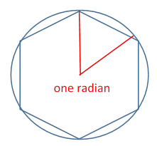
Recall that an ordinary angle is the ratio of the length of circle subtending that angle at the center of the circle to the radius. The natural unit of measure is the radian, defined as the angle subtended by an arc of the circle of length one radius. Since the distance all the way round is $2\pi r,$ that’s just over six radians, so one radian in a little less than the angle subtended by one side of a regular hexagon inscribed in the circle.  In our usual units, that’s a bit less than 60˚, in fact about 57˚.

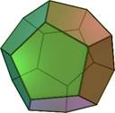
Now, just as a circle can have arcs with lengths measured in radians, a spherical surface can have areas measured in steradians, or squared radians. The area of a spherical surface is $4\pi r^2$, one steradian is the solid angle subtended by an area $r^2$ so the whole surface is $4\pi$ steradians (just as the whole circle is $2\pi$ radians), and one steradian is a little less than the solid angle subtended by one face of a regular  dodecahedron (which has twelve sides).  

An area $A$ on the surface of a sphere of radius $r$ subtends a solid angle $A/r^2$ (steradians) at the center of the sphere.

Consider now an arbitrary smooth closed surface, with a charge $q$ at the origin inside the surface. Take an incremental surface element $d\overrightarrow{A}$ at distance $r$ from the origin. The electric flux through this element is

$$\overrightarrow{E}\cdot d\overrightarrow{A}=\frac{1}{4\pi {\epsilon }_0}q\frac{\overrightarrow{r}\cdot d\overrightarrow{A}}{r^3}.$$

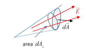
Remembering that by definition the vector describing an area is in a direction perpendicular to that area, the dot product $\overrightarrow{r}\cdot d\overrightarrow{A}=rd{A}_{\perp }$ where $A_{\perp }$ is the projection of the area $d\overrightarrow{A}$ on to a plane perpendicular to $\overrightarrow{r}.$ Now, the infinitesimal area $d{A}_{\perp }$ is on the surface of a sphere of radius $r$ centered at the charge, and subtends a solid angle $d\Omega =d{A}_{\perp }/r^2$ at the charge.  Therefore, the electric flux

$$\overrightarrow{E}\cdot d\overrightarrow{A}=\frac{1}{4\pi {\epsilon }_0}q\frac{\overrightarrow{r}\cdot d\overrightarrow{A}}{r^3}=\frac{1}{4\pi {\epsilon }_0}q\frac{rd{A}_{\perp }}{r^3}=\frac{1}{4\pi {\epsilon }_0}qd\Omega ,$$ 

and integrating over the whole surface

$${\displaystyle \underset{S}{\int }\overrightarrow{E}\cdot d\overrightarrow{A}}=\frac{1}{4\pi {\epsilon }_0}q{\displaystyle \int d\Omega }=\frac{q}{{\epsilon }_0}.$$ 

To summarize: for a point charge $q,$ and an arbitrary closed smooth surface $S,$ ${\displaystyle \underset{S}{\int }\overrightarrow{E}\cdot d\overrightarrow{A}}=\frac{q}{{\epsilon }_0}$  if the charge is inside the surface, and is zero if the charge is outside. (Sketch the mathematically equivalent fluid flow to see why.) But we know from Gauss’ law that

${\displaystyle \underset{S}{\int }\overrightarrow{E}\cdot d\overrightarrow{A}}={\displaystyle \underset{V}{\int }\overrightarrow{\nabla }\cdot \overrightarrow{E}{d}^{3}r.}$ 

This can only be consistent if the point charge, say at ${\overrightarrow{r}}_1,$ is represented mathematically by the charge distribution $\rho \left(\overrightarrow{r}\right)=q\delta \left(\overrightarrow{r}-{\overrightarrow{r}}_1\right),$ and

$\overrightarrow{\nabla }\cdot \overrightarrow{E}=\rho \left(\overrightarrow{r}\right)/{\epsilon }_0.$ 

We’ve only established this explicitly for a point charge, but any charge distribution can be written as a sum of points in the limit, so the linearity of electrostatics assures us this must be a general result.

(If you feel uncomfortable working with the delta function, it might help to represent it as a small sphere carrying uniform surface charge.)

The Electrostatic Potential

The electric field at $\overrightarrow{r}$ from a point charge $Q$ at ${\overrightarrow{r}}_1$ is, in SI units

$$\overrightarrow{E}\left(\overrightarrow{r}\right)=\frac{1}{4\pi {\epsilon }_0}Q\frac{\overrightarrow{r}-{\overrightarrow{r}}_1}{{\left|\overrightarrow{r}-{\overrightarrow{r}}_1\right|}^3}.$$ 

Hence the work done against the electric field of the point charge $Q$  in moving a small charge $q$ from a point $A$ to a point $B$ is (taking now the position ${\overrightarrow{r}}_1$ of $Q$ as the origin)

$W_{\text{path A}\to \text{B}}=-q{\displaystyle \underset{{\overrightarrow{r}}_A}{\overset{{\overrightarrow{r}}_B}{\int }}\overrightarrow{E}\cdot \overrightarrow{ds}}=-\frac{Qq}{4\pi {\epsilon }_0}{\displaystyle \underset{{\overrightarrow{r}}_A}{\overset{{\overrightarrow{r}}_B}{\int }}\frac{\widehat{r}\cdot \overrightarrow{ds}}{r^2}}=-\frac{Qq}{4\pi {\epsilon }_0}{\displaystyle \underset{r_A}{\overset{r_B}{\int }}\frac{dr}{r^2}}=\frac{Qq}{4\pi {\epsilon }_0}\left(\frac{1}{r_B}-\frac{1}{r_A}\right).$

(As usual, $\widehat{r}$ denotes a unit vector in the direction of $\overrightarrow{r}.$ )

This is of course very familiar from the gravitational analogy$—$the crucial point is that the work done depends only on the radii (from $Q$ ) of the endpoints, not on the path taken, and therefore one can define a potential energy function of position, so that the potential energy of a charge $q$ at point $\overrightarrow{r}$ is $q\phi \left(\overrightarrow{r}\right)$, and the potential at $\overrightarrow{r}$ from the point charge $Q$ at the origin is

$$\phi \left(\overrightarrow{r}\right)=\frac{Q}{4\pi {\epsilon }_{0}r}.$$ 

The principle of superposition for electric fields trivially extends to potentials, since the integral is linear in the field, so the potential from a spatial distribution of charge is

$$\phi \left(\overrightarrow{r}\right)=\frac{1}{4\pi {\epsilon }_0}{\displaystyle \int \frac{\rho \left({\overrightarrow{r}}^{\prime }\right)}{\left|\overrightarrow{r}-{\overrightarrow{r}}^{\prime }\right|}}{d}^3{r}^{\prime },$$ 

where the density function $\rho \left({\overrightarrow{r}}^{\prime }\right)$ can include delta functions for point charges.

Getting the Electric Field from the Potential

It’s often easier to compute the potential than find the electric field for a given charge distribution, since, for the field, one must sum over vectors, for the potential, it’s just addition of numbers.  So, suppose we’ve found the potential as a function of position:  how do we use it to get the electric field at a particular point $\left(x,y,z\right)$?

Writing the formula for potential difference between two points separated by an infinitesimal distance in the $x$ direction,

$\phi \left(x+dx,y,z\right)-\phi \left(x,y,z\right)=-{\displaystyle \underset{\left(x,y,z\right)}{\overset{\left(x+dx,y,z\right)}{\int }}\overrightarrow{E}\cdot \overrightarrow{ds}}=-E_{x}dx,$

it follows that

$$E_x=-\frac{\partial \phi \left(x,y,z\right)}{\partial x}.$$

That is,

$\overrightarrow{E}=-\overrightarrow{\nabla }\phi ,\text{ or }\overrightarrow{E}=-\text{grad}\phi .$

In other words, the electric field in a particular direction is the negative of the slope of the potential in that direction: it’s worth looking at a couple of examples to see this in action.

Poisson’s and Laplace's Equations

Putting together $\overrightarrow{E}=-\overrightarrow{\nabla }\phi$ and $\overrightarrow{\nabla }\cdot \overrightarrow{E}=\rho \left(\overrightarrow{r}\right)/{\epsilon }_0$ gives Poisson’s equation

${\nabla }^2\phi =-\rho /{\epsilon }_0.$ 

In the charge free region, it’s of course ${\nabla }^2\phi =0,$ this is sufficiently common and important to merit its own name: Laplace’s equation.

Of course, ${\nabla }^2\phi \left(\overrightarrow{r}\right)=-\rho \left(\overrightarrow{r}\right)/{\epsilon }_0,$  must be consistent with $\phi \left(\overrightarrow{r}\right)=\frac{1}{4\pi {\epsilon }_0}{\displaystyle \int \frac{\rho \left({\overrightarrow{r}}^{\prime }\right)}{\left|\overrightarrow{r}-{\overrightarrow{r}}^{\prime }\right|}}{d}^3{r}^{\prime }.$ 

This follows from

$${\nabla }_{\overrightarrow{r}}{}^2\frac{1}{\left|\overrightarrow{r}-{\overrightarrow{r}}^{\prime }\right|}=-4\pi \delta \left(\overrightarrow{r}-{\overrightarrow{r}}^{\prime }\right).$$ 

(Check it by integrating over a small spherical surface!)

Electrostatic Potential Energy

The work done to bring a point charge $q_i$ from infinity to $\overrightarrow{r}$ in the presence of a fixed charge distribution $\rho \left({\overrightarrow{r}}^{\prime }\right)$ (which does not extend to infinity) is

$W_i=q_i\phi \left(\overrightarrow{r}\right)=\frac{1}{4\pi {\epsilon }_0}{\displaystyle \int \frac{q_i\rho \left({\overrightarrow{r}}^{\prime }\right)}{\left|\overrightarrow{r}-{\overrightarrow{r}}^{\prime }\right|}}{d}^3{r}^{\prime },$ 

and for a set of fixed point charges:

$W_i=q_i\phi \left(\overrightarrow{r}\right)=\frac{1}{4\pi {\epsilon }_0}{\displaystyle \sum _{j=1}^{n-1}\frac{q_i{q}_j}{\left|\overrightarrow{r}-{\overrightarrow{r}}_j\right|}}.$ 

So what is the total potential energy of a set of point charges?

This means the energy necessary (and it could be negative), beginning with all the charges at infinity, to move them up one at a time to their assigned positions.

The total work needed, and therefore the electrostatic potential energy of the configuration, is

$W=\frac{1}{4\pi {\epsilon }_0}{\displaystyle \sum _{i=1}^{n-1}{\displaystyle \sum _{j<i}\frac{q_i{q}_j}{\left|{\overrightarrow{r}}_i-{\overrightarrow{r}}_j\right|}}},$ 

usually written

$W=\frac{1}{8\pi {\epsilon }_0}{\displaystyle \sum _{i,j\left(i\ne j\right)}\frac{q_i{q}_j}{\left|{\overrightarrow{r}}_i-{\overrightarrow{r}}_j\right|}}$ 

with unrestricted sums on $i,j,$ except, obviously, excluding $i=j.$ Notice the extra factor of 2 in the denominator, since summing over all $i,j$ counts each pair potential energy twice.

For a continuous charge distribution, the potential energy is

$W=\frac{1}{8\pi {\epsilon }_0}{\displaystyle \int \frac{\rho \left(\overrightarrow{r}\right)\rho \left({\overrightarrow{r}}^{\prime }\right)}{\left|\overrightarrow{r}-{\overrightarrow{r}}^{\prime }\right|}}{d}^{3}r{d}^3{r}^{\prime },$ 

(no need to worry about $\overrightarrow{r}={\overrightarrow{r}}^{\prime }$ as long as the charge density is finite$—$you should check this, though).

The potential energy can be written equivalently as

$W=\frac{1}{2}{\displaystyle \int \rho \left(\overrightarrow{r}\right)\phi \left(\overrightarrow{r}\right)d^{3}r,}$ 

and therefore from Poisson’s equation

$W=-\frac{{\epsilon }_0}{2}{\displaystyle \int \phi \left(\overrightarrow{r}\right){\nabla }^2\phi \left(\overrightarrow{r}\right)d^{3}r,}$ 

then by integrating over all of space (so the only boundary surface is at infinity, where the integrand will have gone to zero),

$W=\frac{{\epsilon }_0}{2}{\displaystyle \int {\left(\overrightarrow{\nabla }\phi \left(\overrightarrow{r}\right)\right)}^2{d}^{3}r}=\frac{{\epsilon }_0}{2}{\displaystyle \int {\left|\overrightarrow{E}\right|}^2{d}^{3}r}.$ 

So, in an electrostatic situation, we can think of the energy as residing in space, with this density, the square of the local value of the field.  Obviously, the total energy is positive, and, in contrast to the potential and the field, the local energy density is nonlinear: the electric field energy of a uniformly charged unit sphere with charge $2Q$ is four times that of the same sphere carrying charge $Q.$

Exercise:  For the two cases of a uniform solid sphere of charge, and a sphere with charge uniformly distributed over the surface, find the total electrostatic energy by both methods: $W=\frac{1}{2}{\displaystyle \int \rho \left(\overrightarrow{r}\right)\phi \left(\overrightarrow{r}\right)d^{3}r,}$ and $W=\frac{{\epsilon }_0}{2}{\displaystyle \int {\left|\overrightarrow{E}\right|}^2{d}^{3}r}.$ 

Note that this equivalence can't work for genuine point charges (if such could exist): the integral of field energy would diverge around each point. In our formulas for electrostatic energy of a set of point masses, this "self-energy" term is ignored.  Hence the derivation of energy in terms of the squared field integral is really only valid for point charges once we've set aside this (infinite!) self-energy. Think about how this works for two equal point charges initially infinitely separated, then brought close to each other. What about opposite charges?

previous  index  next