7. Electrostatics II: Conductors, Green's Theorem, Green's Functions
The Story So Far…
After Coulomb determined the inverse square law of electrical force in 1785, his French theoretical colleagues Lagrange, Laplace, Poisson and others applied the newly developing calculus techniques to analyzing the electric field from any given distribution of charge. As discussed in the last lecture, the experimental findings of the inverse-square law and the linearity (just add the fields from different charges) led them to define a function The local electric field is the gradient of this function, and the function satisfies Poisson’s equation,
with the local charge density. (The function was first called the potential by George Green, many years later.)
For a given charge distribution the solution is
For the important special case of a charge-free region, the potential satisfies Laplace's equation.
written
(Historical aside: As the French were creating this elegant mathematical analysis of electrostatics, nothing much was going on in English physics, perhaps surprising because a century earlier the English had completely dominated the subject, thanks to Newton, who’d invented calculus, and then explained the solar system with his universal theory of gravitation. But at the same time Newton invented calculus, so did Leibniz, on the continent, essentially independently, and Leibniz constructed a notation more amenable to use by ordinary mortals. Heated arguments about priority ensued for at least a century, with the unfortunate result that the English did not appreciate the French achievements. Cambridge was a backwater for a long time.)
Anyway, Poisson’s equation, if we can solve it, tells us the electric potential, and therefore its gradient the electric field, from any arbitrary charge distribution.
So doesn’t that solve electrostatics? What more do we need to know? Keep reading.
Conductors
 In fact, electrostatics was a very fashionable subject at the
time (around 1800). The sparks you can get brushing your hair (or some clothes)
in winter were the inspiration for brushing machines, designed to capture friction-generated
charge and store it in a jar, all well-insulated of course, to raise the
potential to the point where large sparks could be produced, or people could be
electrically shocked (believed to be of therapeutic value,
but mainly for
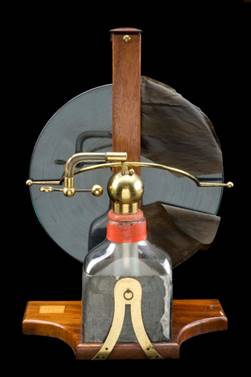
amusement). Here is a picture of such a
machine (by Robert Bancks, Science Museum, London). The disk in back rotates,
there are brushes at the ends of the long horizontal brass bar that capture electric charge, which is stored in the jar. (Production of
electricity from friction between the right materials had been known since
antiquity.)
In fact, electrostatics was a very fashionable subject at the
time (around 1800). The sparks you can get brushing your hair (or some clothes)
in winter were the inspiration for brushing machines, designed to capture friction-generated
charge and store it in a jar, all well-insulated of course, to raise the
potential to the point where large sparks could be produced, or people could be
electrically shocked (believed to be of therapeutic value,
but mainly for
amusement). Here is a picture of such a
machine (by Robert Bancks, Science Museum, London). The disk in back rotates,
there are brushes at the ends of the long horizontal brass bar that capture electric charge, which is stored in the jar. (Production of
electricity from friction between the right materials had been known since
antiquity.)
The details are not important for our purposes: what is
important is to realize that if we want to analyze what’s going on
mathematically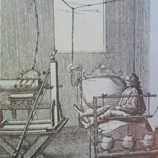 (for example to find the field strength and therefore
possibility of a spark) we need to know the charge distribution, and even if we know the total charge on the spheres, that
isn’t enough, because since they are conductors, the charge will move around,
depending on the local electric field from the other charges.
(for example to find the field strength and therefore
possibility of a spark) we need to know the charge distribution, and even if we know the total charge on the spheres, that
isn’t enough, because since they are conductors, the charge will move around,
depending on the local electric field from the other charges.
Bottom line: if we know the charge distribution, we can calculate the fieldbut with conductors present, we likely don’t know the charge distribution.
A Very Simple Example
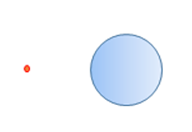
To strip the problem to its essence, let us consider placing a single positive point charge a short distance away from a fixed conducting sphere, the sphere having no net charge. Since it’s a conductor, charge on the surface will flow as the point charge is put in place, so in electrostatic equilibrium there will be excess negative charge on the side facing the positive point charge.
Now how do we find the field?
We don’t know the charge distribution, but we do know something: the electric potential has the same value over the whole spherical surface, or charge would flow, since it’s a conductor, and we’re doing electrostatics.
The very simplest case would be to connect the sphere to ground, in which case we would have over the whole surface (note that the sphere would now have net negative charge coming up from the ground). For this case, then, the mathematics is clear: we must solve Poisson’s equation in the space excluding the conductor, so is just the delta function for the positive charge, but we require the boundary condition on the surface of the conductor.
Summarizing: If we have an electrostatic configuration that includes conductors as well as charges, we must now solve Poisson's equation for the potential subject to given boundary conditions.
Actual solution turned out to be quite tough even for simple geometries, and progress was slow. Poisson himself solved the problem of two charged conducting spheres near each other: this involved infinite series, and virtuoso mathematical effort went into establishing convergence. Gauss found some important results in 1839, and at about the same time a new generation in Cambridge was finally beginning to move on from Newton’s methods, and appreciate the Continental achievements.
George Green: The Breakthrough
Then something completely unexpected happened. In 1845, twenty-one year old William Thomson (the future Lord Kelvin, at Cambridge), aided by his exam coach William Hopkins, finally tracked down a paper he’d heard mentioned by a colleague, privately printed by an obscure miller in Nottingham, one George Green, seventeen years earlier, in 1828. It presented an elegant technique for solving many of these notorious problems!
(Trivia: Hopkins was a very famous coach, an important part of this Cambridge mathematics revival: his students included Stokes and Maxwell. At that time, the word “coach” (inspired by the then rapid road transit between Cambridge and London) was used exclusively for expert math tutors, later it was extended to athletics.)
Incredibly, Green’s work was a substantial improvement on the French achievements. As Thomson remarked, Green’s approach made possible solution of important problems which the traditional methods would never have managed. In fact, Green’s methodsat the present day very well-known as Green’s functionsare an essential set of tools over a vast area of theoretical physics. To give one example, Julian Schwinger, in giving an account of his Nobel-prize-winning calculation of the magnetic moment of the electron wrote (in 1993) that the calculation was by “George Green and I”. Schwinger had learned about Green's functions (in E&M) while working on radar during World War II. As he demonstrated, the functions also work fine in quantum mechanics, where they are now universally used.
George Green himself (born 1793) had only one year of schooling (when he was eight), he was too busy operating his father’s mill. However, the business prospered and later he could afford to spend some time in a remarkably good library privately sponsored in Nottingham. It is possible that he came across Poisson’s work there (he cites it in his 1828 paper), and maybe he bought French mathematics journals or books. There was one other person in Nottingham who might have helped, a local headmaster (John Toplis) who translated some of Laplace’s work in 1814. Nevertheless, it struck William Thomson (Lord Kelvin to be), and everybody since, as almost unbelievable that someone so far from an academic setting, with almost no formal schooling, working by himself, could so greatly extend the impressive work of the French school. Sad to report, George Green died before his work was appreciated.
Green’s Identity and Green’s Theorem
You might think that a substantial contribution to the solution of Poisson’s equation with arbitrary boundary conditions in three dimensions would be highly technical and tough to follow, but in fact Green’s methods are quite straightforwardit was just that no one had thought this way before.
As a warmup to establish notation, consider a point charge in empty space.
We know that for any closed surface having the origin inside. That is to say, with
provided the volume integrated includes the origin, and is zero otherwise. That is, the integrand is zero everywhere except at the origin, but if the volume integrated over includes the origin, the integral is finite, and has a definite value.
This is precisely our definition of the delta function! Matching the sides of the equation,
(Green made extensive use of this identity, but of course didn’t call it a delta function, that’s Dirac’s notation. He also didn’t use vectors, they were invented later in the nineteenth century by Heaviside and Gibbs. Green just wrote out components.)
Now on to the general problem of finding the electric field from a given fixed charge density, including possible point charges, plus a set of conductors.
Each conductor has either a specified total charge, or is fixed at a given potential.
What we don't know at this stage is how the charge is distributed on the conductor(s) (all we know is it's on the surface(s) in this static case), so obviously we can’t just solve Poisson’s equation to find the potential.
Green’s First Identity
Here's how Green attacked the problem. He began with the divergence theorem for a general vector field
and applied it to a vector field of the form
where are arbitrary scalar fields.
It’s easy to check that
and
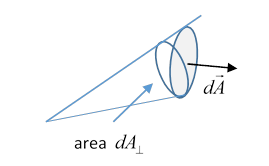
where is the normal derivative at the surface, directed out from and is the element of area, the magnitude of . Putting these in the divergence theorem,
This is often called Green’s first identity.
Now the trick is to write the same identity with interchanged, and subtract one from the other, to get Green’s Theorem (a.k.a. Green’s second identity):
To apply this identity to electrostatics problems, we take to be the electrostatic potential from some volume charge distribution in the presence of conducting closed surfaces (this is what we’re trying to find, we prime the variables for later convenience), and for a preliminary exercise we take
Therefore
Putting these into Green’s theorem gives, for a given fixed in and integrating over (both volume and surface)
Putting in the 's from the previous equation, we find, rearranging (check this!),
Let’s interpret this equation term by term.
The first term is just the ordinary potential from the charges in the volume (meaning not on the boundary surfaces).
The first surface termthe normal (and only) component of the electric field at the surface, is from the charge layer on the surface (there being no electric field pointing from the surface inwards, since in electrostatics the potential is constant throughout the volume of the conductor). Therefore this is just the contribution to the potential from the charge densities on the conducting surfaces. (Be careful with the sign of this term: we began with the divergence theorem, where the surface integral has the small area vectors pointing outwards from the integration volume, meaning into the conductors.)
The second surface
term in the equation is equivalent to a dipole
layer of strength :
obviously not physically present, so what does this mean? The mathematical derivation is correct, it
must mean something. Assuming that the
surface is an ordinary conductor, so the potential is constant over the whole surface, then this
term represents a dipole layer of uniform
strength,
 an element having dipole moment Therefore (applying our result from earlier, in
lecture 2) the potential at is proportional to the solid angle subtended by the surface at which would be zero for a closed surface, unless it surrounds the point in
question, in which case it would contribute (the cancel).
an element having dipole moment Therefore (applying our result from earlier, in
lecture 2) the potential at is proportional to the solid angle subtended by the surface at which would be zero for a closed surface, unless it surrounds the point in
question, in which case it would contribute (the cancel).
Physically, then, the potential at a point in the volume is the sum of the potentials from the charge in the volume and the charge distribution on the surfaces, plus that last term: and that term only contributes if the whole system is inside a conducting surface, in which case the potential anywhere is just that from the enclosed charges plus the overall potential , say, of the surrounding surface, which is effectively the background potential inside the surface.
The essential point: the only effect of a closed surface covered with a uniform dipole layer is to generate a constant potential difference between the inside and the outside. (Physically, there is a delta-function perpendicular electric field within the dipole layer.)
So, adding the three terms together, this exercise has told us something we already knew: the total electric potential at any point is the sum of that from the volume charge, that from the surface charge layers, and an overall constant being that of the enclosing boundary conductor (if any). What, exactly, was the point? The point was to get familiar with Green’s theorem, which has many further uses we’ll now investigate.
Introducing Green’s Function
This is where Green provided the key: in the derivation above, we took
satisfying
But the derivation would still have worked if we replaced with a more general function provided only that
This is a Green’s function. Evidently, it must have the form
where throughout the volume.
As discussed earlier, surface charges are generated or rearranged in response to the presence of the point charge, and the term is the potential change from this rearrangement of charges, which depends on the given boundary conditions: do these conductors have fixed charges, or are they at fixed potentials, or even some mix?
(You may be aware that in practice, the field from these surface charges is sometimes equivalent to that from a simple charge distribution outside the spacefor example, if the space is bounded by a plane, a single “image charge” in the half plane beyond the conducting surface is enough. If you’re not familiar with this, don’t worry, we’ll get to it shortly.)
With this new function we can write the potential anywhere in the volume as
(The is for Green.)
Nowimportant!staring at the right hand side of this equation, we see that if we can find a that is zero when is on the surface(s) and we know its normal derivative there, we can find just from knowing on Furthermore, since we’re taking all these surfaces to be conductors, will be just a constant on each of them. This is progresswe just have to find
Boundary Conditions: Dirichlet and Neumann, and the Corresponding Green’s Functions
As with any differential equation, to solve for we must specify boundary conditions.
The two boundary conditions used here are:
Dirichlet, when the value of the function is specified on the boundary, and
Neumann, when the normal derivative is given at the boundary.
The Dirichlet Green‘s Function
We define the Dirichlet Green‘s function by requiring the boundary condition:
for on the surface in
Looking back at the equation above for we see that using this the first surface integral vanishes, andprovided we’ve actually found a satisfying this at any point in the volume can be calculated from input data throughout the volume, plus just on all the bounding surfaces, we don’t also need on the surfaces .
That is to say,
You might wonder if a function necessarily exists satisfying in the volume and for on the surface in Green himself pointed out that it does: it’s just the potential from a unit point charge at when the surfaces are grounded.
Furthermore, this means that is the charge density induced on the conducting surface at from a unit charge at
The Neumann Green’s Function
The Neumann boundary condition ( on the surfaces?) is slightly trickier, remember the general form of the Green’s function is so for a surface enclosing we must have meaning we can’t require everywhere on that boundary, which would eliminate the second surface integral in the above equation for The best we can do to simplify the Neumann Green’s function is to make its normal derivative constant on the boundary,
for on
( also denotes the total surface area.) This gives the solution
Note that we only have this trouble (of not being able to put ) on surfaces surrounding so if our problem has various closed surfaces but is outside all of them, we have no problem, for in using Green’s methods to go from a volume to an integral over bounding surfaces, the only one enclosing will be a sphere (say) at infinity, where the average value of can be taken zero.
Uniqueness of the Solution with Dirichlet or Neumann Boundary Conditions
First we'll establish that if we do find a solution, it's the only one. Suppose we have a volume with a set of boundary surfaces, which for now we’ll take to be conductors, plus some charge distribution (point charges or densities of charge) inside the volume. If we specify the charge distribution, and also the potentials on the conducting surfaces, the electric field will be uniquely defined. Intuitively, this seems certain, but we’ll prove it below anyway.
Recall from above that specifying the potential on the boundary of the space is the Dirichlet boundary condition, specifying the normal derivative (the electric field here) is the Neumann boundary condition.
Either way, we’ll show that the solution to the equation is unique.
To prove there's only one solution, suppose there are two, and is the difference between them, so throughout the volume, and either (Dirichlet) or (Neumann) on the boundary. Then, from Green’s first identity:
putting we have
and therefore, since if the surface integral on the right vanishes, which it does for either the Dirichlet or the Neumann boundary conditions, or even for mixed boundary conditionsDirichlet on some boundaries, Neumann on others. Hence is constant through the system, the electric field difference is zero everywhere.
Formal Solution of Electrostatic Boundary-Value Problems with Green’s Functions
Recalling that the Dirichlet boundary condition is specifying the value of the potential on the boundary, we define the Dirichlet Green’s function by
for on in
If we can actually find satisfying this, the above equation for is much easier to solve: the first surface integral vanishes, and at any point in the volume can be calculated from input data throughout the volume, plus just on all the bounding surfaces (for conductors, constant on each one). We don’t need on the surfaces.
That is to say,
A Surface on Which the Potential is Nonuniform
Consider for example a sphere in which the northern hemisphere and the southern hemisphere are both conductors, but there is a thin band of insulator around the equator, and the two halves are at different potentials. How do we find the potential from this charged object?
Looking at the equation above, we see the first thing we need is the Green’s function for outside the sphere, satisfying and on the spherical surface.
This is nothing but the electrostatic potential from a unit charge placed at when the spherical surface is grounded.
Now the outward derivative of the electric potential, is precisely the charge density at on the grounded surface induced by the point charge at , let’s call it
The equation for the potential (from the end of the previous section, but with zero volume charge) now becomes:
This is a remarkable result (found by Green himself) because it’s true even if varies over the surface! That is to say, if we know the formula for the distribution of charge on a grounded conducting sphere in the presence of a single point charge at P outside it (which we’ll find in the next lecture), we can immediately write down the potential at that same point P generated by having different parts of the surface held at different potentials.
To further check this equation for the potential, note first that because on the right hand side only appears in and there is no space charge To verify that approaches the local on approaching the surface is a little more tricky, we’ll give a fuller discussion in the next lecture. Essentially, as the point charge approaches the surface it induces a charge distribution on the surface that approaches a delta function. Close enough, the surface can be treated as a plane, and, as discussed in the next lecture, the induced charge is equivalent to a point image charge at the reflection of the approaching charge, going to a delta function in the limit.
Note: we’ve taken here a spherical surface as an example, but the result is good for any shape closed smooth surface.
The Green’s Function is Symmetric
The Dirichlet Green’s function is symmetric,
This is proved by substituting in Green’s theorem
Since both are Dirichlet functions in this case, they are identically zero in the surface integral on the right-hand side, and on the left use to do the volume integrals.
Jackson remarks that this symmetry of “merely represents the physical
interchangeability of the source and observation points”. Well, yes, but that
is not at all obvious! Suppose we put a
 single charge at .
The cylinder is grounded to ensure it stays at zero potential, so opposite
charge to will flow from the ground and be most
concentrated on the cylinder close to .
The resulting electric field will be quite complicated, and have some value at Now start again: put the charge at let’s say on the axis of the cylinder. Now the
induced charge distribution on the cylinder will be cylindrically symmetric,
quite different from the previous case. The theorem tells us that in this case,
the potential at is that
same This is obvious?
single charge at .
The cylinder is grounded to ensure it stays at zero potential, so opposite
charge to will flow from the ground and be most
concentrated on the cylinder close to .
The resulting electric field will be quite complicated, and have some value at Now start again: put the charge at let’s say on the axis of the cylinder. Now the
induced charge distribution on the cylinder will be cylindrically symmetric,
quite different from the previous case. The theorem tells us that in this case,
the potential at is that
same This is obvious?
Force on the Surface of a Charged Conductor
Suppose that the local surface charge density is An element of the surface will itself generate outward electric fields But we know there’s no field inside the conductor, so the charges elsewhere must be generating a local field and therefore a force tending to push the element outwards. If the force does on fact push the area a distance outwards (think of a charged soap bubble) the electric field does work That must mean this amount of potential energy has disappeared from the electric field: but that was exactly the amount in the volume of field that has disappeared (remember there’s zero field inside the conductor, the disappearing outside field is . This is one element’s contribution to expanding the whole conducting surface, we can’t just lift one bit).