previous  index  next 

9. Green’s Reciprocation Theorem

Michael Fowler, University of Virginia

What It Is

One simple theorem George Green published in his 1828 paper is his Reciprocation Theorem. (This is Jackson's term, Wikipedia calls it reciprocity.) It seems almost trivial, but often leads to surprising results with very little effort.  Here it is:

Consider two different volume and surface charge distributions, in the same identical geometry.

Charge distribution A has volume charge density ${\rho }_A\left(\overrightarrow{r}\right)$ and boundary surface charge densities ${\sigma }_A\left(\overrightarrow{r}\right),$ generating electrostatic potential ${\phi }_A\left(\overrightarrow{r}\right).$

In that same space (meaning with the same surfaces) charge distribution B, with densities ${\rho }_B$, ${\sigma }_B$ would give potential ${\phi }_B\left(\overrightarrow{r}\right).$ 

Then the Reciprocation Theorem is:

$${\displaystyle \underset{V}{\int }{\rho }_A{\phi }_{B}dV+{\displaystyle \underset{S}{\int }{\sigma }_A{\phi }_{B}da}}={\displaystyle \underset{V}{\int }{\rho }_B{\phi }_{A}dV+{\displaystyle \underset{S}{\int }{\sigma }_B{\phi }_{A}da}}.$$

In words:  If the A charge densities were at rest in the B potential, the total potential energy would be the same as that of the B charge densities held at rest in the A potential.

To prove it, we’ll just consider volume charges (the surface charges could be taken as volume charges in a thin layer limit anyway).

Then

$${\phi }_B\left(\overrightarrow{r}\right)=\frac{1}{4\pi {\epsilon }_0}{\displaystyle \underset{V}{\int }\frac{{\rho }_B\left({\overrightarrow{r}}^{\prime }\right)}{\left|\overrightarrow{r}-{\overrightarrow{r}}^{\prime }\right|}}$$

 and

$${\displaystyle \underset{V}{\int }{\rho }_A\left(\overrightarrow{r}\right){\phi }_B\left(\overrightarrow{r}\right)d^{3}r}=\frac{1}{4\pi {\epsilon }_0}{\displaystyle \underset{V}{\int }\frac{{\rho }_A\left(\overrightarrow{r}\right){\rho }_B\left({\overrightarrow{r}}^{\prime }\right)}{\left|\overrightarrow{r}-{\overrightarrow{r}}^{\prime }\right|}}{d}^{3}r{d}^3{r}^{\prime }.$$

But this is symmetric in A, B, proving the theorem: it’s that simple!

Earnshaw’s Theorem from the Reciprocation Theorem

Earnshaw’s theorem is often stated simply as: In a charge-free region, the potential cannot have a maximum or minimum. (Because locally the field in all directions would have to point all inwards or all outwards, so nonzero divergence, meaning there must be charge present.)

A more informative version is: in a charge-free region, the potential at a point is the same as the average potential on any spherical surface centered at that point, provided only that the spherical surface is itself within the charge-free region.

To prove this using the Reciprocation Theorem, take:

System A:  the existing setup, with charge distribution ${\rho }_A\left(\overrightarrow{r}\right)$ all outside the region of interest, generating potential ${\phi }_A\left(\overrightarrow{r}\right).$

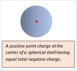
System B:  a spherical surface, radius $R,$ with uniform surface charge density $\sigma$, the total surface charge being $4\pi R^2\sigma =-Q,$ and a point charge $+Q$ at the center of the sphere.

The spherical surface is taken to be in the charge-free region of system A.

The B system, the charged sphere plus the equal but negative central point charge, gives zero potential outside the sphere (which is where all the A system charge is), so

${\displaystyle \int {\rho }_A\left(\overrightarrow{r}\right)}{\phi }_B\left(\overrightarrow{r}\right)=0.$

 Therefore from the theorem ${\displaystyle \int {\phi }_A\left(\overrightarrow{r}\right){\rho }_B\left(\overrightarrow{r}\right)}=0,$ and taking the center of the sphere as the origin for convenience, this becomes, integrating over the area of the spherical surface (and cancelling out $Q$ from both sides):

$$\frac{1}{4\pi R^2}{\displaystyle \int {\phi }_A\left(\overrightarrow{r}\right)R^{2}d\Omega }={\phi }_A\left(0\right).$$

Note:  if this looks too easy, there are many more difficult proofs on the web.

Exercise:  Suppose we take a new system B: a sphere centered at the origin with surface charge density proportional to the coordinate $z.$ We replace the center point charge with a point dipole, such that the potential from this system is zero outside the sphere. System A is as before: what does the Reciprocation Theorem tell you this time? Hint: you can think of that surface charge as two equally-sized solid spheres of charge of opposite sign, their centers a very small distance apart.

 Revisiting an Earlier Result Using the Reciprocation Theorem

We established in the Electrostatics II lecture that if different parts of a spherical surface are held at different potentials, the consequent potential at any point P in space outside the sphere can be found by integrating over the spherical surface with a weighting factor equal to the density of induced charge on a perfectly conducting grounded sphere with a unit charge at the point P.

In fact, this result follows immediately from the reciprocation theorem!

For

${\displaystyle \underset{V}{\int }{\rho }_A{\phi }_{B}dV+{\displaystyle \underset{S}{\int }{\sigma }_A{\phi }_{B}da}}={\displaystyle \underset{V}{\int }{\rho }_B{\phi }_{A}dV+{\displaystyle \underset{S}{\int }{\sigma }_B{\phi }_{A}da}},$

consider two systems A, B with identical geometry: just a sphere plus one point outside it.

System A is our spherical surface divided into parts held at different potentials, labeled by the variable potential ${\phi }_A\left({\overrightarrow{r}}^{\prime }\right),$ ${\overrightarrow{r}}^{\prime }$ being any point on the surface of the sphere, and system A also includes the point P, position $\overrightarrow{r}$ say, at which we want to find the potential from the charge distribution on the spherical surface (but there is no volume charge in A). 

System B is the geometrically identical sphere, but now a fully connected conducting surface, grounded and so at zero potential, and now there is a unit charge at the point P, that is, ${\rho }_B\left(\overrightarrow{r}\right)=\delta \left(\overrightarrow{r}-{\overrightarrow{r}}_{\text{P}}\right).$ 

The left-hand side of the equation above is identically zero: ${\rho }_A=0$ in the volume, ${\phi }_B=0$ on the surface.

The right-hand side, using ${\rho }_B\left(\overrightarrow{r}\right)=\delta \left(\overrightarrow{r}-{\overrightarrow{r}}_{\text{P}}\right),$ gives ${\phi }_A\left(\overrightarrow{r}\right)=-{\displaystyle \underset{S}{\int }{\sigma }_B\left({\overrightarrow{r}}^{\prime }\right){\phi }_A\left({\overrightarrow{r}}^{\prime }\right)da},$ where ${\sigma }_B\left({\overrightarrow{r}}^{\prime }\right)$ would be the surface charge density induced at ${\overrightarrow{r}}^{\prime }$ on a grounded conducting sphere by unit charge at $\overrightarrow{r}.$

Note also that this proof generalizes from a conducting sphere to any closed conducting surface.  

Symmetry of the Dirichlet Green's Function

We’ve shown the Dirichlet Green’s function is symmetric, 

$G_D\left(\overrightarrow{r},{\overrightarrow{r}}^{\prime }\right)=G_D\left({\overrightarrow{r}}^{\prime },\overrightarrow{r}\right).$

This also follows easily from the Reciprocation Theorem: take two systems A, B having the same set of grounded conducting surfaces, one with a single unit charge at $\overrightarrow{r},$ the other with a single unit charge at ${\overrightarrow{r}}^{\prime }$. Now, by definition, $G_D\left(\overrightarrow{r},{\overrightarrow{r}}^{\prime }\right)$ is the potential at $\overrightarrow{r}$ from the single unit charge at ${\overrightarrow{r}}^{\prime }$ plus the charges induced on the grounded surfaces, and vice versa.  Symmetry follows from The Theorem. (The result is certainly not intuitively obvious: think of an odd shaped conductor, say a sphere but with a tall thin conical "mountain" somewhere. Now put $\overrightarrow{r}$ just above the mountain peak, ${\overrightarrow{r}}^{\prime }$ above the plane on the other side.)

Exercise:  Write this out explicitly, in terms of ${\rho }_A,{\phi }_A,{\rho }_B,{\phi }_B.$ 

previous  index  next