8. The Image Method in Electrostatics

Introduction

The presentation of Green’s functions in the preceding lecture was based on a paper George Green wrote in 1828, privately printed, and read by almost nobody until William Thomson (the future Lord Kelvin) stumbled on it in 1842. Thomson realized its importance, and created the image technique as an easy way to construct Green’s functions for some simple geometries, in particular a plane and a sphere.

Point Charge and Grounded Conducting Plane

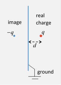
Let’s start with the simplest problem: a charge $q$ at $(d, 0, 0)$ to the right of the infinite grounded plane $x = 0.$ The grounded plane is of course the boundary, on which $φ = 0,$ so this is a Dirichlet problem: we need to find the potential in the half space to the right of the plane, generated by the point charge plus the charge induced on the conducting plane.

From the uniqueness theorem (presented in the previous lecture), if we can find any charge distribution in the left-hand half-space that, together with the existing point charge on the right, gives $φ = 0$ everywhere on the plane $x = 0,$ it will give the correct potential everywhere in the right-hand half space, the region we’re interested in.

As William Thomson pointed out, the appropriate charge distribution for this geometry is actually very simple: just a single “image” charge $- q$ placed at the mirror image point. Check it out: every point in the plane is equidistant from the equal positive and negative charges, so is at zero potential.

Now recall we defined the Green’s function $G (\vec{r}, {\vec{r}}^{'})$ by saying that $\frac{G (\vec{r}, {\vec{r}}^{'})}{4 π ε_{0}}$ is the potential at point $\vec{r}$ from a single unit charge at the point ${\vec{r}}^{'} .$ And, as we established in the last lecture, the Dirichlet Green’s function (the one relevant here) is symmetric between $\vec{r}$ and ${\vec{r}}^{'} .$ (Sorry about the $1 / 4 π ε_{0}$ : it's in Jackson, but not all books.)

Evidently the Green’s function for this image problem is just

$G_{D} (\vec{r}, {\vec{r}}^{'}) = \frac{1}{|\vec{r} - {\vec{r}}^{'}|} - \frac{1}{|\vec{r} - {\vec{r}}^{'}_{refl}|}$ .

We’ve added the subscript $D$ because, being zero on the boundary, this is, by definition, the Dirichlet Green’s function (discussed at length in the previous lecture), and the general formula for the potential anywhere in the volume $—$ that would be the physical volume, the half of space to the right of the plane in the diagram above, where the charge is $—$ includes a term from the boundary surfaces:

$φ (\vec{r}) = \frac{1}{4 π ε_{0}} \int_{V} G_{D} (\vec{r}, {\vec{r}}^{'}) ρ ({\vec{r}}^{'}) d V - \frac{1}{4 π} \int_{S} \frac{\partial G_{D} (\vec{r}, {\vec{r}}^{'})}{\partial n^{'}} φ ({\vec{r}}^{'}) d a^{'} .$

In this case, though, the potential $φ ({\vec{r}}^{'})$ is zero on the boundary $—$ the grounded plane $—$ so the second term vanishes, leaving the simple result.

It’s worth emphasizing what a breakthrough the image method was. Together with the crucial uniqueness theorem, it renders this problem almost trivial. Previously, it would have been solved by laboriously computing the induced charge on the plane, using its circular symmetry and balancing the force on one element of charge from all the others. OK, doable, but problems involving more images, for example the interaction of two charged separated conducting spheres, needed (pre-image!) mind numbing amounts of computation.

Charge Distribution on the Plane

The charge density at a point on the conducting plane is given by the local value of the normal directed electric field

$\frac{\partial G_{D} (\vec{r}, {\vec{r}}^{'})}{\partial n^{'}} = E_{⊥} ({\vec{r}}^{'}) = σ ({\vec{r}}^{'}) / ε_{0} .$

(In fact the field must be normal to the surface for a conductor in an electrostatics problem $—$ if there's a component parallel to the surface, then from continuity there will be a similar parallel field inside the conductor, charge will move, and this isn't electrostatics until things settle down.)

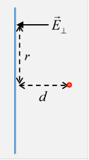
Taking the charge to be a distance $d$ from the plane, remembering the contribution from the image charge (the factor 2 in the equation below), and measuring $r$ on the plane from an origin directly below the charge, with the perpendicular component of the field denoted by $E_{⊥}$ (and dropping the prime to reduce clutter),

$\frac{σ (\vec{r})}{ε_{0}} = E_{⊥} (\vec{r}) = - \frac{1}{4 π ε_{0}} \cdot 2 \cdot \frac{q}{r^{2} + d^{2}} \cdot \frac{d}{\sqrt{r^{2} + d^{2}}} = - \frac{1}{4 π ε_{0}} \frac{2 q d}{{(r^{2} + d^{2})}^{3 / 2}},$

$σ (r, d) = - \frac{1}{2 π} \frac{q d}{{(r^{2} + d^{2})}^{3 / 2}} .$

Just to check, the total charge is

$σ_{total} = - \frac{q d}{2 π} \int_{0}^{\infty} \frac{2 π r d r}{{(r^{2} + d^{2})}^{3 / 2}} = - q .$

Exercise: Show that in the limit as the charge moves closer and closer to the plane, the induced charge distribution approaches a delta function.

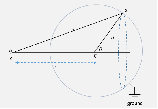
Point Charge and Grounded Conducting Sphere

The problem we just did, the point charge and the conducting plane, is clearly a special case of a point charge and a conducting sphere (the sphere having infinite radius), and we approach it with the same strategy.

The idea is to place a negative "image" charge somewhere so that the potentials from charge + image exactly cancel on the spherical surface. Obviously the image charge must have different magnitude from the initial charge, otherwise the zero potential surface would be the plane problem we just solved.

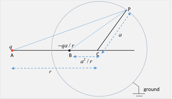
This cancellation will only work if for every point on the surface, the ratio of distances from the two fixed charges is the same. Really, we don't have to visualize this in three dimensions: just take a plane that includes the line from the charge at A to the center C of the sphere. Is there a point B on this line such that for every point P on the circle the ratio of lengths PA/PB is the same?

If yes, make the ratio of the charge strengths the inverse of this distances ratio, and the total potential on the spherical surface will be zero. But: is there such a point?

Luckily, the ancient Greeks solved the problem: P lies on the circle of Apollonius, defined as the set of points with a given distance ratio from two given fixed points $—$ it turns out to be a circle.

In the language of our problem, if the original charge at A is a distance $r$ from the center of the sphere of radius $a,$ and $r > a,$ the image charge has strength $- q a / r$ and is a distance $a^{2} / r$ from the center of the sphere, on the line to the original charge. To reduce clutter, we'll write

$\frac{r}{a} = λ .$

Now look at the diagram: we’ll prove that these two charges add to give zero potential everywhere on the circle.

We need a little geometry: for any point P on the sphere, from the diagram, the triangles APC, BPC are similar (they have a common angle, and the sides containing that angle have lengths with the same ratio) so the ratio of the distances from P to the charge and the image charge PA/PB = PC/BC = $r / a = λ .$

This ratio is independent of where P is on the sphere, so if the charges are in the ratio $- 1 / λ,$ meaning $q_{image} = - q a / r,$ the potential will be zero over the whole surface.

Since the Dirichlet Green’s function for the space outside the sphere is defined as the electric potential at $\vec{r}$ from a point unit charge at ${\vec{r}}^{'}$ (well, multiplied by $4 π ε_{0}$ ) subject to $φ = 0$ on the boundary, exactly the condition we have, it follows that for the spherical geometry

$G_{D} (\vec{r}, {\vec{r}}^{'}) = \frac{1}{|\vec{r} - {\vec{r}}^{'}|} - \frac{a / |{\vec{r}}^{'}|}{|\vec{r} - a^{2} {\vec{r}}^{'} / {|{\vec{r}}^{'}|}^{2}|} .$

(Historical trivia footnote: this problem was solved by William Thomson shortly after he saw Green’s paper in 1845. Thomson was home schooled by his father, a math teacher who later became a math professor at the University of Glasgow. Both would have been completely familiar with Greek geometry, in particular Apollonius, so this would not have been a difficult problem. (Griffiths fantasizes about the first person to solve this problem: “Presumably, he (she?) started with an arbitrary charge at an arbitrary point inside the sphere” … well, no.)

Charge Distribution on the Sphere

The way to find the charge distribution, exactly as for the conducting plane, is to find the electric field from charge + image charge at a point on the spherical surface, then recall that in the real problem, that must be the field outside the sphere, and, with no field inside, it must be the local surface charge density (divided by $ε_{0}$ , of course) , that is, $E_{⊥} = σ / ε_{0} .$

As before, we know that the field must be normal to the surface, it’s a conductor and this is electrostatics, but nevertheless it’s reassuring to check.

As in the diagram, we take a point P on the spherical surface, distance $s$ from charge $q$ at A and distance $s / λ$ from charge $- q / λ$ at B.

We’ll analyze the electric fields at P from the two charges, but instead of the usual horizontal and vertical components, we’ll take in the horizontal direction AC and the radial direction CP. This makes sense, because the radial component is directly related to the charge density on the surface.

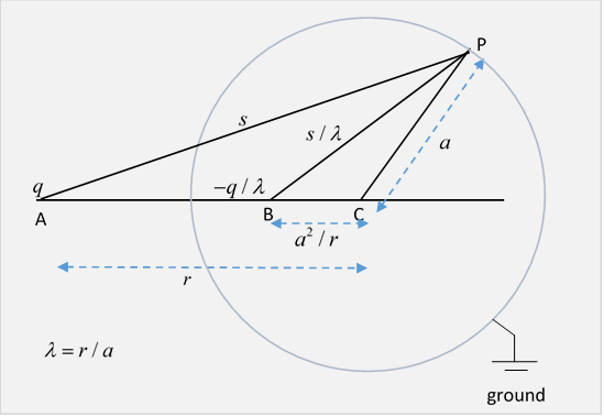
Furthermore, the geometry of the diagram (look at it), the lengths of the sides of the triangles, make it easy to find the ratios of these components to the total force.

Field components at P from $q$ at A:

$(E_{A horizontal}, E_{A radial}) = \frac{1}{4 π ε_{0}} \cdot \frac{q}{s^{2}} \cdot (\frac{r}{s}, \frac{a}{s}) .$

Field components at P from $- q a / r$ at B: $(E_{B horizontal}, E_{B radial}) = - \frac{1}{4 π ε_{0}} \cdot \frac{q / λ}{{(s / λ)}^{2}} \cdot (\frac{a^{2} / r}{s / λ}, \frac{a}{s / λ}) .$

Using $r = λ a$ it is easy to check that the first components cancel, as they must, and the second add to give an electric field

$E_{⊥} = \frac{1}{4 π ε_{0}} \cdot \frac{q}{s^{3}} \cdot (1 - λ^{2}) a = \frac{1}{4 π ε_{0}} \cdot \frac{q}{s^{3}} \cdot \frac{(a^{2} - r^{2})}{a},$

so the induced charge density, everywhere negative ( $r > a$ ), is simply proportional to the inverse cube of the distance s from the point charge:

$σ (s) = - \frac{1}{4 π} \cdot \frac{q}{s^{3}} \cdot \frac{(r^{2} - a^{2})}{a} .$

It’s worth emphasizing that this induced charge is the normal derivative of the Green's function: we're going to find this valuable in solving some quite different problems!

$σ (s) = ε_{0} E_{⊥} = - ε_{0} q \frac{\partial G (\vec{r}, {\vec{r}}^{'})}{\partial n^{'}} .$

(We have to be careful about the sign of $n^{'}$ : it points outward from the volume integrated over.)

Aside: using this charge distribution to solve a potential problem.

We’ll interrupt the narrative briefly here to point out that having found this charge distribution, we can now solve a problem mentioned in the Electronics II lecture, the potential at a point in space from a charged sphere on which different areas of the surface are held at different potentials. The relevant equation is

$φ (\vec{r}) = - \frac{1}{4 π} \int_{S} \frac{\partial G_{D} (\vec{r}, {\vec{r}}^{'})}{\partial n^{'}} φ ({\vec{r}}^{'}) d a^{'} = \int_{S} σ (\vec{r}, {\vec{r}}^{'}) φ ({\vec{r}}^{'}) d a^{'},$

and here, with $|\vec{r} - {\vec{r}}^{'}| = s,$ $σ (s) = - \frac{1}{4 π} \cdot \frac{q}{s^{3}} \cdot \frac{(r^{2} - a^{2})}{a} .$ Jackson gives a specific example: two hemispheres at different potentials. We give details at the end of this lecture.

To check the total induced charge (which had better equal the value of the image charge) we need to integrate the charge density over the whole spherical surface:

The total induced charge (remember this is a sphere, P is on a circle of equal induced charge, shown dashed)

$\begin{matrix} \int_{sphere} σ (r) d A = - \frac{q}{4 π} \cdot \frac{(r^{2} - a^{2})}{a} \cdot \int_{0}^{π} \frac{2 π a \sin θ d θ}{{(r^{2} + a^{2} + 2 a r \cos θ)}^{3 / 2}} \\ = - \frac{q}{4 π} \cdot \frac{(r^{2} - a^{2})}{a} \cdot 4 π a \cdot \frac{1}{2 a r} \cdot (\frac{1}{r - a} - \frac{1}{r + a}) \\ = - q \cdot \frac{a}{r} = - \frac{q}{λ} . \end{matrix}$

Exercise: Suppose the grounded conducting sphere suddenly becomes an insulator, with all the surface charge now stuck in place. Then suppose the outside charge $q$ is removed to infinity.

Describe the electric field (a) outside the sphere, and (b) inside the sphere.

The answer to (a) is that it must of course be identical to that from the image charge $—$ this makes it obvious that the attractive force on the charge $q$ from the total surface charge density $σ$ must be precisely that from a single charge, the image charge. But what about (b)?

Point Charge with Charged, Isolated, Conducting Sphere

We've just established that a point charge $q$ distance $r$ from the center of a conducting sphere of radius $a < r,$ the sphere being held at $φ = 0$ , gives an electric field equal to that from $q$ plus an image charge $- q / λ, λ = r / a,$ at a distance $a^{2} / r$ from the center of the sphere, in the same direction as the original charge.

To find the electric field from a non-grounded sphere carrying total charge $Q,$ we simply add to charge + image another point charge $Q + q / λ$ at the point corresponding to the center of the sphere. This will ensure the surface is still an equipotential, though not of course at potential zero.

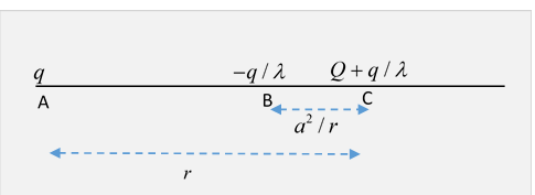
To find the force on $q$ from the charged isolated sphere, add the image force to that from the new central charge:

Remembering that $1 / λ = a / r,$ the electric force on $q$ towards the sphere is

$F = \frac{q}{4 π ε_{0}} [\frac{q a / r}{{(r - (a^{2} / r))}^{2}} - \frac{Q + q a / r}{r^{2}}]$ .

This can be rearranged to separate out the $Q, q a / r$ terms:

$F = - \frac{q}{4 π ε_{0} r^{2}} [Q - \frac{q a^{3} (2 r^{2} - a^{2})}{r {(r^{2} - a^{2})}^{2}}] .$

It’s worth noting the general form of this force: as the charge $q$ approaches the sphere’s surface, $r \to a$ , the force becomes infinitely attractive, $\frac{q^{2}}{4 π ε_{0}} \frac{1}{4 {(r - a)}^{2}}$ , entirely from the image charge. At distances $r ≫ a$ , the image charge contribution is of order $1 / r^{3},$ so the $q Q / r^{2}$ term dominates.

If $Q$ and $q$ are both positive, there is a distance at which there is zero electric force on $q$ from the sphere, and the larger $Q$ is relative to $q$ , the closer this is to the surface.

Point Charge Near a Conducting Sphere at Fixed Potential

The external charge $q$ and its image result in the sphere having zero potential, so to bring the sphere’s potential to $V$ we must add a term $V a / r$ to $φ$ (outside the sphere). This is equivalent to placing a charge $Q = 4 π ε_{0} V a$ at the center of the sphere. In this case, the total charge on the sphere is $Q - q a / r$ , and so varies as the outside charge $q$ is moved to different radial distances $r$ . This sphere must therefore be connected to a constant potential battery, and will adjust its total charge as $q$ moves.

Conducting Sphere in a Uniform Electric Field by the Method of Images

A conducting sphere of radius $a$ is centered at the origin, and the uniform electric field is provided by taking large, faraway charges $Q$ at $z = - R$ and $- Q$ at $z = R .$

Taking the limit $R \to \infty$ keeping $Q / R^{2}$ constant, the external field strength at the sphere is

$E_{0} = \frac{1}{4 π ε_{0}} \cdot \frac{2 Q}{R^{2}} .$

We know from earlier that the charge $Q$ at $z = - R$ will induce an image charge $- Q a / R$ at the point

$z_{image} = - a^{2} / R,$

so the two far distant large charges induce an image dipole at the center of the sphere, of strength

$p = \frac{Q a}{R} \cdot \frac{2 a^{2}}{R} = 2 a^{3} \frac{Q}{R^{2}} = 4 π a^{3} ε_{0} E_{0} .$

That is, two equal and opposite image charges are generated, an infinitesimal distance apart. Obviously, no net charge is induced on the sphere, so it doesn’t matter if it’s grounded or insulated.

Recall now from an earlier lecture that the electric field from a dipole is

${\vec{E}}_{dipole} (\vec{r}) = \frac{1}{4 π ε_{0}} \frac{3 \hat{\vec{r}} (\hat{\vec{r}} \cdot \vec{p}) - \vec{p}}{r^{3}} .$

Now $\vec{p} = 4 π a^{3} ε_{0} {\vec{E}}_{0}$ , so the field outside the sphere is

$\vec{E} (\vec{r}) = {\vec{E}}_{dipole} + {\vec{E}}_{0} = \frac{3 \hat{\vec{r}} (\hat{\vec{r}} \cdot {\vec{E}}_{0}) - {\vec{E}}_{0}}{r^{3}} a^{3} + {\vec{E}}_{0} .$

Far away, the dipole field falls as $1 / r^{3},$ leaving just ${\vec{E}}_{0},$ but right at the spherical surface $r = a$ the constant field is exactly canceled by the second term in the dipole field, leaving only a radial electric field, as we must of course have for the conducting surface. The field magnitude is $3 (\hat{\vec{r}} \cdot {\vec{E}}_{0}),$ so the surface charge is

$σ = ε_{0} E = 3 ε_{0} E_{0} \cos θ .$

Here’s one way to look at it: the field from a solid uniformly filled sphere of charge is $q / 4 π ε_{0} r^{2}$ outside, exactly the same as from a point charge $q$ at the center. Therefore, the field of a dipole strength $q d$ at the origin is the same outside the sphere as that of a $+ q$ sphere centered at the origin plus a $- q$ sphere centered at the infinitesimal (in the limit) position $- d .$ But for these two spheres, the net charge will cancel except for a surface layer of thickness $d \cos θ$ (see figure).

The volume charge density in the sphere is given by $\frac{4}{3} π a^{3} ρ = q,$ so the charge layer has strength $ρ d \cos θ = 3 q d \cos θ / 4 π a^{3} .$ Now $q d = p = 4 π a^{3} ε_{0} E_{0},$ from above, and the result follows.

It must also be that this induced charge density creates a uniform electric field inside the sphere to cancel exactly the external constant electric field. That is also easy to see from representing it as two almost overlapping spheres, as we’ll now show.

The electric field inside a sphere uniformly charged throughout its volume is linear in distance from the center, like gravity inside the Earth, and therefore has the form $\vec{E} = \frac{q}{4 π ε_{0} a^{2}} \frac{\vec{r}}{a} .$ Therefore, the field from the two spheres of charge infinitesimally displaced is

$\vec{E} = \frac{q}{4 π ε_{0} a^{2}} \frac{\vec{r}}{a} - \frac{q}{4 π ε_{0} a^{2}} \frac{\vec{r} + \vec{d}}{a} = - \frac{q \vec{d}}{4 π ε_{0} a^{3}} = - \frac{\vec{p}}{3 ε_{0} V},$

$V$ being the volume of the sphere, and $\vec{p} = 4 π a^{3} ε_{0} {\vec{E}}_{0}$ , so the layer of surface charge creates a field exactly opposite to the external field.

(Note for future use: a polarized dielectric sphere really is like two slightly relatively displaced spheres of charge, and if it has total dipole moment $\vec{p},$ it has polarization density $\vec{P} = \vec{p} / V,$ so its polarization generates an electric field ${\vec{E}}_{pol} = - \vec{P} / 3 ε_{0} .$ )

More Images…

The examples analyzed above have a charge and a single image $—$ but there can be more! Consider a charge placed at a point P near the intersection of two conducting planes, both connected to ground and so having $φ = 0.$ From the diagram, it’s clear that to have zero potential on both planes, we need three images, not just two.

This can be extended to three dimensions: in a corner where three infinite perpendicular conducting planes intersect, say, we’ll need seven image charges.

A point charge between two parallel plane conductors generates an infinite series of images, as does a system consisting of just two charged spheres. It’s clear that all this can lead to an infinite number of homework problems…

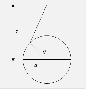
Hemispheres at Different Potentials

Again, the result of our Green's function calculation is that if different parts of a spherical surface are held at different potentials, the potential at any point P in the space outside the sphere can be found by integrating the given potential over the spherical surface with a weighting factor equal to the density of induced charge on a perfectly conducting grounded sphere with a unit charge at the point P.

One specific example (done in Jackson) is a spherical shell with a thin band of insulator around the equator, the two halves at potentials $\pm V$ respectively.

We’ll find the potential on the $z$ axis, meaning the line through the two poles, perpendicular to the equatorial plane.

From the top half, the contribution to

$φ (\vec{r}) = \frac{1}{4 π} \int_{S} φ ({\vec{r}}^{'}) \frac{a (r^{2} - a^{2})}{{|\vec{r} - {\vec{r}}^{'}|}^{3}} d Ω$

$φ_{top} (\vec{r}) = \frac{1}{4 π} \int_{θ = 0}^{π / 2} V \frac{2 π a (z^{2} - a^{2}) \sin θ d θ}{{(z^{2} + a^{2} - 2 a z \cos θ)}^{3 / 2}} = - V (\frac{z^{2} - a^{2}}{z}) [\frac{1}{\sqrt{z^{2} + a^{2}}} - \frac{1}{z - a}],$

(with the standard change of variables to $μ = \cos θ, d μ = - \sin θ d θ$ )

and adding the similar contribution from the bottom half,

$φ (z) = V [1 - \frac{(z^{2} - a^{2})}{z \sqrt{z^{2} + a^{2}}}] = V [1 - (1 - \frac{a^{2}}{z^{2}}) {(1 + \frac{a^{2}}{z^{2}})}^{- \frac{1}{2}}] ≅ V [\frac{3}{2} \frac{a^{2}}{z^{2}} - \frac{7}{8} \frac{a^{4}}{z^{4}} + \dots]$

In Jackson's discussion of this problem, he goes on to address the more general case of the potential off the axis, where the integrals can only be done by expanding the denominator in a power series and then attacking it term by term. But, as we shall see when we get to Legendre polynomials, this effort is completely unnecessary $—$ the axial symmetry means that we can expand the potential in Legendre polynomials multiplied by the appropriate power of the radius, so once we know the potential on the axis, extending into all of space is trivial. Jackson’s equation (2.27) (where $x$ oddly means $r$ ) follows immediately from the equation for $φ (z)$ above.

Finally: this approach is not restricted to a spherical conductor. If you can find the Dirichlet Green’s function for a conductor, and therefore the induced surface charge when the conductor is grounded and a unit charge is placed at a point P outside, then you can find the potential at P from different parts of the conductor’s surface being held at different potentials by using the surface integral as above.

previous index next