previous  index  next 

16.  Conformal Mapping

    Michael Fowler, UVa

Introduction

Conformal mapping is really just another term for what we've been doing above$—$but expressed rather differently. It’s formulated in terms of mapping from the usual complex plane $z=x+iy$ to another complex plane $w=u+iv$ (or the other way) by means of a function analytic (differentiable) in the region of interest,

$w=f\left(z\right).$

For $z_0$ in the region, and $w_0=f\left(z_0\right),$ for small deviations within the region

$w-w_0\cong \left(\frac{df}{dz}\right)\left(z-z_0\right)=A{e}^{i\alpha }\left(z-z_0\right).$

So locally the grid of orthogonal $x,y$ lines goes to a grid of orthogonal $u,v$ lines, scaled by a factor $A$ and rotated through an angle $\alpha ,$ but the important point is it’s still an orthogonal grid, the right angles are preserved$—$this is what is meant by a conformal mapping.  Notice in the above equation, if the small number $z-z_0$ is turned through 90 degrees, then $w-w_0$ will correspondingly turn through 90 degrees.  Furthermore, for an analytic function of a complex variable the real and imaginary parts separately satisfy the 2D Laplace equation, meaning they represent the electrostatic potential for some arrangement of charges positioned outside the domain of analyticity.

This means that if we can solve a 2D electrostatic problem for some configuration of conductors in the $z$-plane, making an analytic transformation to the $w$-plane automatically solves the potential problem for the transformed shapes of conductors.  

Conformal mappings and invariance are very common in the theory of phase transitions, string theory, etc.  String theory is actually a conformal two-dimensional theory.

Mapping the Real Axis to the Unit Circle

A simple example is a mapping from the real axis to the unit circle, taking as usual $z=x+iy$ and $w=u+iv,$ 

$$z=\frac{w-i}{w+i}.$$

This maps the real $w$-axis on to the unit circle $\left|z\right|=1.$ Check that $w=\pm \infty$ goes to $z=1,$ $w=0$ goes to $z=-1,$ and $w=\pm 1$ to $z=\mp i.$   Note also that

$$w=-i\frac{z+1}{z-1}.$$

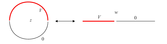
Let's see how this connects the split cylinder in the $z$-plane with potential $V$ for the top half and zero for the bottom half (discussed in lecture 15) to the problem of infinite flat conducting plates in the $w$-plane, with potential $V$ for $u<0,$ and zero for $u>0$ (discussed in lecture 14) .

The correct potential for the $w$-plane problem (see lecture 14) is ${\phi }_w\left(w\right)=\left(V/\pi \right)\mathrm{Im}\ln w.$

To try to reduce confusion, we will (temporarily) put a subscript on the potential to remind us which picture we’re looking at. 

In the $z$-plane we define the potential ${\phi }_z\left(z\right)$ by ${\phi }_z\left(z\right)={\phi }_w\left(w\left(z\right)\right).$

That is, under the mapping $w\to z$, ${\phi }_z\left(z\right)$ is assigned the same value ${\phi }_w\left(w\right)$ had at the corresponding point $w,$ meaning

$${\phi }_z\left(z\right)=\left(V/\pi \right)\mathrm{Im}\ln w=\left(V/\pi \right)\mathrm{Im}\ln \left(-i\frac{z+1}{z-1}\right).$$

Equipotentials of course must map (both ways) into equipotentials: check one or two for yourself.  For example, what about the real $z$-axis?

Maxwell's Mapping for a Parallel Plate Capacitor Edge

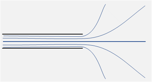
What makes the mapping approach worthwhile is well illustrated by Maxwell’s use of it to solve an important problem: what, exactly, do the equipotentials look like near the edge of a parallel plate capacitor?

Maybe like this?

 There are two distinct regions:

1.   Deep inside (far to the left), the equipotentials must look like those between infinite plates$—$far enough back, the fact that the plates come to an end can make little difference.

2.   On the other hand, well outside the plates, meaning at distances much greater than the distance between the plates, it will look like the field from plates at potentials $0,V$ coming together at an angle very close to $2\pi .$ We discussed this two-plates-at-an-angle configuration earlier:  for angle $2\pi ,$ the equipotentials are lines radiating out from the join, the (orthogonal) electric field lines tend to concentric circles far away.

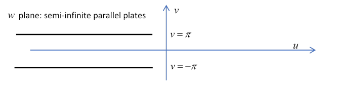
Maxwell began with infinite parallel plates

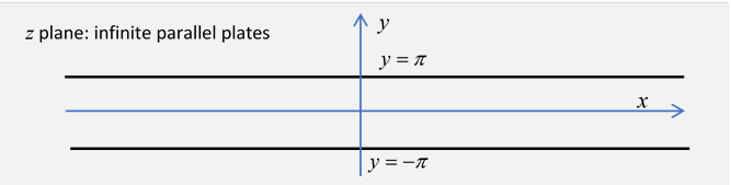
Taking the plate separation conveniently equal to $2\pi ,$ Maxwell used the transformation

$w=u+iv=z+e^z$

to map the space between the plates to the whole complex plane.

In terms of real and imaginary parts,

$u=\left(x+e^x\cos y\right),v=\left(y+e^x\sin y\right).$

Notice that this has the features we want: for $x$ large and negative, it tends to $w=z,$ meaning that moving to the left we find a field between the plates looking almost the same as for infinite plates, whereas for large positive $x,$ the $z\to w$ map gives equipotentials  (maps of lines of constant $y$ ) radiating out from the end of the plates, the exponential term completely dominates.

The central line, $y=0,$ goes to $v=0,$ we have a symmetric mapping, but it’s not linear$—$look how $u$ relates to $x,$ pretty linear for $u$ negative, but really taking off for $u$ positive and increasing! 

Now let’s look at nonzero positive $v.$ Not much going on for $v$ negative, the exponential terms are tiny, but when $x$ becomes positive and increasing the exponential term finally takes over, and as $x$ continues to increase, the equipotential tends to a straight line at an angle $v$ to the axis. As we approach the upper plate, this angle tends to $\pi ,$  so the lines are fanning out in all directions: we’ve mapped the region between the plates in the $z$ -plane to the whole $w$-plane! 

In particular, the equipotential infinitesimally below the top plate turns through $\pi$ at the end of the plate, and goes back to $-\infty$ infinitesimally above the plate. 

Exercise:  draw these equipotentials. 

Exercise:  In the original (infinite plates) scenario, consider a perpendicular line from one plate to the other to the far right (large positive $x$ ).  That’s a field line.  What does it go to under Maxwell’s mapping to the $w$-plane? 

Trivia note:  Maxwell actually drew these equipotentials himself, and so well that his drawing is used as the cover for his classic book on E&M in the Dover edition.

Field of a Conducting Strip: The Sine Function Mapping

The System

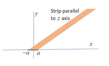
Here we consider the electric field from a long straight charged wire along the $z$-axis, but instead of the usual cylindrical shape (circular cross section) we take it the wire is a long strip of metal, of breadth $2a,$ say, and of negligible thickness, so we can take the 2D cross section to be just a line in the $xy$ plane, on the $x$-axis from $-a$ to $a.$ 

In the $xy$ -plane, for distances $r\gg a$ from the wire, we expect the field to be close to that from a round cylindrical wire. However, very close to the surface of the wire ( $r\ll a$ ), it will approximate the field from a charged plane.  To see quantitatively how it goes from one to the other, we create the field using a conformal mapping (plus some hindsight).

The Mapping

We begin with a much simpler system: the field above a uniformly charged plane, then we map it into the one we want.

For this charged plane system, in the (Cartesian) $z=0$ plane, we label the horizontal and vertical axes $u,v$ and switch to a complex variable representation,

$$w=u+iv.$$

The field above the uniformly charged plane is uniform, so the equipotentials are just horizontal lines in the $u,v$ plane, lines of constant $v,$ and the field lines are vertical lines of constant $u.$

We now restrict our attention to the real axis between $-\pi /2$ and $+\pi /2$ and the part of the plane above it, that is, complex numbers with positive $v$ and $u$ in the range $\left(-\pi /2,\pi /2\right).$

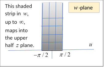
The equipotentials and field lines in this region, of course, form a simple rectangular grid above the uniformly charged plane.

We’re now ready to make a conformal mapping from this $w$-plane to the $z$-plane by the transformation:

$z=a\sin w.$ 

(So $z$ here is a complex variable, not to be confused with the Cartesian coordinate.  Sorry.)

First, what does this do to the real axis part?  It is mapped from $\left(-\pi /2,\pi /2\right)$ to $\left(-a,a\right).$

Exercise: In the $w$-plane, the base was uniformly electrically charged.  Qualitatively, what does the charge distribution look like in the $z$-plane, in particular near the ends?

To see how the rest of the region (the segment of complex plane directly above this stretch of the $u$-axis) transforms,

write

$z=x+iy=a\sin w=a\sin \left(u+iv\right),$

that is,

$x=a\sin u\cosh v,y=a\cos u\sinh v.$

For the constant vertical electric field in the $w$-plane,  the potential is given by $\phi =\mathrm{Im}w=v$, that is, a $w$-plane equipotential will of course be a horizontal line from $u=-\pi /2$ to $\pi /2.$ What happens to this equipotential under the transformation to  the upper half $z=x+iy$ -plane?  It goes to the (upper) half ellipse, constant $\nu ,$ with foci at $\pm a:$

$$\frac{x^2}{{\cosh }^{2}v}+\frac{y^2}{{\sinh }^{2}v}=a^2.$$

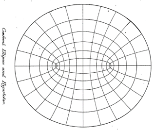
So in the $z$-plane the equipotentials are confocal ellipses, the one corresponding to potential zero is a straight line from $-a$ to $a.$ 

This is the upper half of the field from a charged conducting strip: the degenerate ellipse corresponding to the real axis base in the $w$-plane is an equipotential, so making this an infinitely thin conducting strip will generate this set of elliptical equipotentials, from the uniqueness theorem.  The ellipses can simply be completed for the whole plane. The field lines are the set of confocal hyperbolae

$$\frac{x^2}{{\sin }^{2}u}-\frac{y^2}{{\cos }^{2}u}=a^2.$$

So the transformation has opened up the part of the complex plane above the strip so that it fills the whole upper half plane.

This illustration was drawn by Maxwell himself.

Exercise:  Show that we get essentially the same mapping if we replace sine by cosine, sinh, cosh.

Some insight into the above diagram comes from the inverse mapping,

$$\arcsin \left(z/a\right)=-i\ln \left(\sqrt{1-{\left(z/a\right)}^2}\pm i\left(z/a\right)\right).$$

That is,

$$u+iv=-i\ln \left(\sqrt{1-{\left(z/a\right)}^2}\pm i\left(z/a\right)\right).$$

There are two branch points at $z=\pm a.$ We need to look at the physics to see where to place the branch cut, since the function will be discontinuous on crossing it. Evidently we must put the cut on the real axis from $-a$ to $a,$ and since  $\ln z,$ taken to have a cut along the positive real axis, has a discontinuity $2\pi i$ across the cut, we see the potential $v$ is continuous across the cut (in fact, zero$—$the function in the brackets is of the form $e^{i\theta }$ if $z$ is real and on the cut) but $u$ (called the stream function in hydrodynamics) changes sign, so if we put arrows on the field lines they will, of course, point away from the (positively charged) strip, up and down.

Swapping equipotentials and field lines, we have the field in a gap between two semi-infinite conducting planes held at different potentials: but now we must put the branch cuts from $-\infty$ to $-a,$ and $a$ to $+\infty .$ The field lines, of course, are of opposite sign on the two sides of the charged plate.

Exercise:  Sketch the field lines, with direction arrows, for these two cases.  

previous  index  next