17.  Van der Pauw's Theorem

    Michael Fowler, UVa

Introduction

This is not an electrostatics lecture$—$it’s about steady current flow in two dimensions!  The reason I’ve put it here is because it’s a neat example of the use of complex variable mapping techniques in solving two-dimensional electrical problems, here related to the Hall effect.

Definition of Sheet Conductivity

Given a piece of uniformly thick, but arbitrary shape, semiconductor wafer, how do you measure its conductivity?  (I’m following the presentation in Stone and Goldbart.)

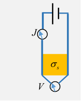
For an effectively two-dimensional material, the sheet conductivity ${\sigma }_s$  is measured by maintaining a voltage difference $V$ between two opposite sides of a square of the material, and measuring the resulting current $J={\sigma }_{s}V.$  The result is independent of the size of the square. (This sheet conductance relates to the ordinary 3D conductance $\sigma$ by ${\sigma }_s=\sigma d,$ $d$ being the sheet thickness.)

Finding Sheet Conductivity for any Shape Sample

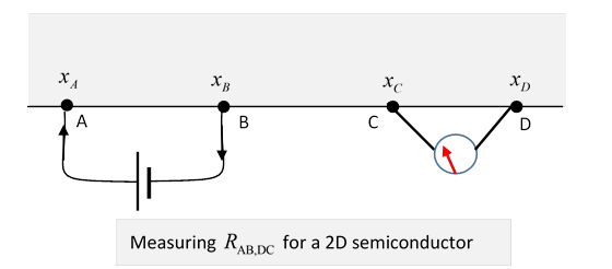
However, Van der Pauw published in 1958 a simple way to find ${\sigma }_s$ for an arbitrarily shaped (but uniform thickness) sample:  attach four (small) contacts to the edge of the sample as shown.

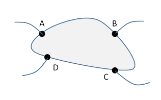
Now pass a current $I_{\text{AB}}$ from A to B, and measure the resulting potential difference $V_{\text{D}}-V_{\text{C}}$.

Define $R_{AB,DC}=\left(V_{\text{D}}-V_{\text{C}}\right)/I_{\text{AB}}.$

Next, pass the current from B to C, giving $R_{\text{BC,AD}}.$ 

Then ${\sigma }_s$ can be found numerically from the equation

$e^{-\pi {\sigma }_s{R}_{AB,DC}}+e^{-\pi {\sigma }_s{R}_{\text{BC,AD}}}=1.$

Where did that come from?  Van der Pauw proved it was true if the sample is half infinite, meaning here it's the upper half plane, then applied Riemann’s mapping theorem, that you could conformally map the upper half plane into the interior of an arbitrary (well, reasonably smooth) shape, and he showed that the formula stays intact!  This kind of thing only works in two dimensions$—$there are far fewer conformal transformations in three dimensions.

To see how this works, we'll begin with the upper half plane:

What is the physics here? We assume Ohm’s law, and steady currents:

$\overrightarrow{J}=-{\sigma }_s\overrightarrow{\nabla }V,\overrightarrow{\nabla }\cdot \overrightarrow{J}=0.$

Therefore ${\nabla }^{2}V=0,$ and this is two dimensions, so for a single (point) source the potential is proportional to $\ln r,r$ being distance from the source. Although we have only a half plane here, it’s clear from the symmetry that the current pattern will be the same as it would be for a full plane (with twice the source and sink strengths).  (Think of the electric field lines in the $x,y$ plane from two uniformly charged lines, one positive, the other same strength negative, parallel to the $z$ axis.)

If we fix the scale by making

$$V\left(x\right)=\ln \frac{x-x_A}{x-x_B},$$

then the current $I_{AB}={\sigma }_s\pi .$  (Because $\overrightarrow{\nabla }V$ is $1/r$ outwards near the source, and the current flows outwards over an angle $\pi .$ )

Defining

$$R_{AB,DC}=\frac{V_D-V_C}{I_{AB}},$$

we see that

$${\sigma }_s\pi R_{AB,DC}=\ln \frac{x_D-x_A}{x_D-x_B}\cdot \frac{x_C-x_B}{x_C-x_A}.$$

and similarly

$${\sigma }_s\pi R_{BC,AD}=\ln \frac{x_A-x_B}{x_A-x_C}\cdot \frac{x_D-x_C}{x_D-x_B}.$$

It’s now simple algebra to prove that

$\exp \left(-{\sigma }_s\pi R_{AB,DC}\right)+\exp \left(-{\sigma }_s\pi R_{BC,AD}\right)=1.$

Riemann’s Mapping Theorem

Now we invoke the Riemann mapping theorem (which was in his 1851 Ph D thesis):

The interior of any simply connected region in the complex plane can be mapped conformally into the interior of the unit circle.

And we’ve already established (in the previous lecture) that the upper half plane can be mapped into the interior of the unit circle.

Therefore, the Van der Pauw theorem proved for the upper half plane can be conformally mapped into any shaped region! We’ll call the region (corresponding to the sample shape) S.

The crucial word is conformal:  there must exist a mapping such that the potential at any point in the upper half plane is the same as the potential at the corresponding point in the sample shape S, the new potential satisfies ${\nabla }^{2}V=0,$ the lines of current flow in the sample map are perpendicular to the equipotentials, etc., the physics is fine.

So the values of the potential at the four sample points are the same as in the upper half plane map, and the value of the current coming from the source is the same. The current and electric field must be parallel to the edge (except at source and sink).

Plausibility Argument for Riemann’s Mapping Theorem

Stone and Goldbart give an interesting physics-type quasi-derivation of Riemann’s theorem, which also stipulates that any interior point in the domain can be mapped to the origin, and an arbitrary orientation angle can be added.

They consider point charge at the origin, the unit circle at zero potential, we know $\phi =-\left(1/2\pi \right)\ln \left|z\right|.$  Now suppose we put a unit point charge in the shape S, keeping the boundary at zero potential. We know there is some corresponding potential ${\phi }_1\left(z\right)$, although it might be hard to find! But it will be the real part of a complex function $\Phi \left(z\right)={\phi }_1+i{\phi }_2.$ Therefore, the mapping we want is $\Phi \left(w\right)=-\left(1/2\pi \right)\ln z.$ The lines of constant $\mathrm{Re}\Phi \left(w\right)$ are the equipotentials, including the shape boundary, and map to the circles around the $z$ plane origin.

The point is that we don’t need to find this map explicitly, only know that it exists, to establish Van der Pauw’s result.

Note: Van der Pauw’s method has been extended to anisotropic materials, varying thickness, etc., admittedly numerically, and is very much in use.  See Wikipedia.