previous  index  next 

25.  Charged Conducting Plane with Circular Hole

    Michael Fowler, UVa

Introduction

Consider a charged conducting sheet in the plane $z=0,$ with a circular hole centered at the origin, circumference $\rho =\sqrt{x^2+y^2}=a.$  This is a reasonable model for the field around a hole in a waveguide, provided the wavelength is much greater than the hole size, so an electrostatic approximation is valid. Outside the waveguide, at distances bigger than the hole size, the field approximates dipole radiation.

For large positive/negative $z,$ Jackson takes constant (perpendicular) electric fields $E_0/E_1.$ We’ll take $E_0=E,E_1=0.$ That is, we take a uniform vertical electric field far above the sheet, from some distant source, but no external charges below the sheet, so the only field below is that from leakage through the hole, and therefore local.  This represents the hole in the waveguide.

Part of Jackson’s purpose in going through this problem is to work with mixed (Dirichlet and Neumann) boundary conditions: the boundary is the plane $z=0,$ for $\rho >0$ the Dirichlet condition $\phi =0$ holds, but in the hole this is no longer true, however the only vertical field, $\partial \phi /\partial n,$ is the known external field, since the induced charge is all at $z=0$ it cannot contribute to the vertical field component in the hole, so the Neumann boundary condition holds.

Jackson points out that textbooks usually ignore problems of this type, and observes that this is because they are much more difficult to handle. He then makes a convincing case: straightforward up to equation 3.178, but then many obscure references and a challenge after 3.184.

But the reason Smythe’s textbook, for example, doesn’t go through this is that there is a much better way to solve this problem: use spheroidal coordinates. OK, there is a learning curve if you’re unfamiliar with them, but it will take less time than really working through Jackson’s solution, and they’re handy for other problems.  

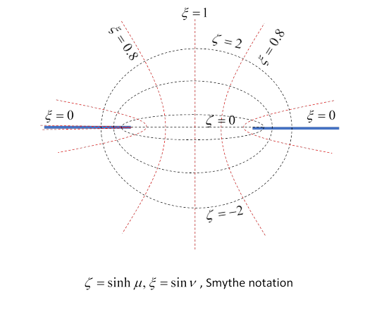
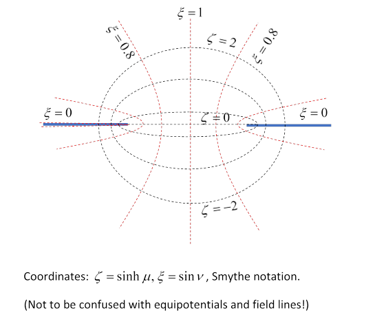
That is, the natural coordinate system for this problem is the same spheroidal coordinates used for the charged conducting disc (and the needle): obviously, the potential is a different function of the coordinates. To quote from the disc lecture, the Cartesian coordinates can be written in terms of (real) parameters $\mu ,\nu$ and azimuthal $\varphi$:

$\begin{array}{l}x=a\cosh \mu \cos \nu \cos \varphi ,\\ y=a\cosh \mu \cos \nu \sin \varphi ,\\ z=a\sinh \mu \sin \nu .\end{array}$

This coordinate system is discussed at length in the conducting disc lecture (and in Wikipedia). 

The curves of constant $\mu$ are ellipses with foci at $\pm a$ (confocal ellipses), the (orthogonal) constant $\nu$ curves are hyperbolas with the same $\pm a$ foci. See the graph in the conducting disc lecture.

The notation is that of Smythe (1950). As will become clear below, the appropriate parameter ranges for this problem are $-\infty <\mu <+\infty ,0\le \sin \nu \le 1.$ (In contrast, in the conducting disc lecture, we took the ranges $0<\mu <+\infty ,-1\le \sin \nu \le 1.$ These choices both ensure continuous parametrization away from the charge.)

Note: These different parameter range choices are exactly equivalent to the placement of branch cuts in the parallel 2D problems of a charged strip and a slit in a conducting plane. Discontinuities in parameters can only occur where there is charge.

Solving with New Parameters: $\xi ,\zeta$

Legendre Solutions

It proves convenient for this problem to go from the parametrization $\left(\mu ,\nu ,\varphi \right)$ used above to $\left(\xi ,\zeta ,\varphi \right)$ where

$\begin{array}{l}\xi =\sin \nu ,\\ \zeta =\sinh \mu .\end{array}$

The azimuthal angle stays the same. The ranges $-\infty <\mu <+\infty ,0\le \sin \nu \le 1$ translate to

$-\infty <\zeta <+\infty ,0\le \xi \le 1.$

In terms of the Cartesian coordinates, via $\left(\mu ,\nu \right)$, we see that

$\begin{array}{l}\rho =\sqrt{x^2+y^2}=a\cosh \mu \cos \nu =a\sqrt{\left(1+{\zeta }^2\right)\left(1-{\xi }^2\right)},\\ z=a\sinh \mu \sin \nu =a\xi \zeta .\end{array}$

From Smythe (or Wikipedia) Laplace’s equation is:

$\frac{\partial }{\partial \xi }\left[\left(1-{\xi }^2\right)\frac{\partial \phi }{\partial \xi }\right]+\frac{\partial }{\partial \zeta }\left[\left(1+{\zeta }^2\right)\frac{\partial \phi }{\partial \zeta }\right]+\frac{{\xi }^2+{\zeta }^2}{\left(1+{\zeta }^2\right)\left(1-{\xi }^2\right)}\frac{{\partial }^2\phi }{\partial {\varphi }^2}=0.$

Separating variables,

$\phi =\Xi \left(\xi \right)Z\left(\zeta \right)\Phi \left(\varphi \right),$

and taking the $\Phi$ eigenvalue to be $-m^2$ as usual, and dividing by $\Xi Z\Phi ,$

$\begin{array}{c}\frac{1}{\Xi }\frac{d}{d\xi }\left[\left(1-{\xi }^2\right)\frac{d\Xi }{d\xi }\right]+\frac{1}{Z}\frac{d}{d\zeta }\left[\left(1+{\zeta }^2\right)\frac{dZ}{d\zeta }\right]=\frac{m^2\left({\xi }^2+{\zeta }^2\right)}{\left(1+{\zeta }^2\right)\left(1-{\xi }^2\right)}\\ =\frac{m^2}{1-{\xi }^2}-\frac{m^2}{1+{\zeta }^2}.\end{array}$

Proceeding just as with spherical harmonics, writing $n\left(n+1\right)$ to represent a (so far) arbitrary constant, we have

$\begin{array}{l}\frac{d}{d\xi }\left[\left(1-{\xi }^2\right)\frac{d\Xi }{d\xi }\right]-\frac{m^2\Xi }{1-{\xi }^2}+n\left(n+1\right)\Xi =0,\\ \frac{d}{d\zeta }\left[\left(1+{\zeta }^2\right)\frac{dZ}{d\zeta }\right]+\frac{m^{2}Z}{1+{\zeta }^2}-n\left(n+1\right)Z=0.\end{array}$

This first equation we’ve seen before!  Recall from the Spherical Harmonics lecture that the associated Legendre Polynomial $P_l^m\left(x\right)$ satisfies

$\left(\frac{d}{dx}\left(1-x^2\right)\frac{d}{dx}+l\left(l+1\right)-\frac{m^2}{1-x^2}\right)P_l^m\left(x\right)=0$

with $l,m$ integers, and the solutions are

$P_l^m\left(x\right)={\left(-1\right)}^m{\left(1-x^2\right)}^{m/2}\frac{d^m}{d{x}^m}{P}_l\left(x\right).$

So this means ${\Xi }_l^m\left(\xi \right)=P_l^m\left(\xi \right)$ is a solution of the first equation, and, furthermore, making the argument pure imaginary, $Z_l^m\left(\zeta \right)=P_l^m\left(i\zeta \right)$ solves the second equation. (Check that!).

So there are solutions are of the form ${\phi }_l^m={\Xi }_{lm}\left(\xi \right)Z_{lm}\left(\zeta \right){\Phi }_m\left(\varphi \right)=P_{lm}\left(\xi \right)P_{lm}\left(i\zeta \right){\Phi }_m\left(\varphi \right).$

Doesn’t that mean we’re done?  Well, no. There are more solutions to these equations: they’re second order differential equations, so they have two solutions.

To quote again from the Spherical Harmonics lecture: for the simplest possible case,  $l=0$ (so $m=0$ too, of course)

 “possible independent solutions are $P_0\left(x\right)=1$ and $P_0\left(x\right)=\ln \left(1+x\right)-\ln \left(1-x\right).$ This second solution, although mathematically OK, is singular at the north and south poles, which are not special points$—$we could have set our coordinate system at any orientation.  So from now on we'll drop singular solutions (for any value of $l$ ).”

But: this reasoning doesn’t carry over to the present problem.  Since $\xi \ge 0,$ and from the diagram we see that the edges of the hole are at $\xi =0,$ knowing as we do that charge can pile up in a singular fashion at the edge of a conductor, evidently we must include possible singular solutions.

The first few singular solutions (known as Legendre Functions of the Second Kind) are:

$\begin{array}{l}{Q}_0\left(x\right)=\frac{1}{2}\ln \frac{1+x}{1-x},\\ Q_1\left(x\right)=\frac{1}{2}x\ln \frac{1+x}{1-x}-1,\\ Q_1^1\left(x\right)=\sqrt{1-x^2}\left(\frac{1}{2}\ln \frac{1+x}{1-x}+\frac{x}{1-x^2}\right).\end{array}$

(See Wolfram.)  

(Note that for pure imaginary argument, $Q_0\left(i\zeta \right)=\frac{1}{2}\ln \frac{1+i\zeta }{1-i\zeta }=i{\tan }^{-1}\zeta .$ )

However, at this point Smythe notes (p 145, top) that the general solution to Legendre’s equation has the form $A{P}_n+B{Q}_n,$ so he goes to $A^{\prime }=A-\frac{1}{2}B\ln (-1)$, which amounts to adding the constant $\frac{1}{2}\ln \left(-1\right)$ to $Q_0,$ thereby switching the sign of the denominator, giving

$Q_0\left(i\zeta \right)=-i{\cot }^{-1}\zeta .$

This $Q_0$ is the same as Morse and Feshbach, p 1328.  This rearrangement doesn’t affect the physics, since the multiplying constants of $P_0,Q_0$ are fixed at the end by matching to known asymptotic behavior. (This is just a warning to be careful in using multiple sources.)

A general solution of the differential equation is a sum of terms ${\Xi }_{mn}{Z}_{mn}{\Phi }_m,$ but our problem has azimuthal symmetry, so only $m=0.$ 

The solution must match a constant downward electric field at large positive $z$ distances.

Recalling that

$\rho =a\sqrt{\left(1+{\zeta }^2\right)\left(1-{\xi }^2\right)},z=a\xi \zeta ,$

 define the distance $r$ from the origin by

$r^2={\rho }^2+z^2.$

At large distances,

$r^2=a^2\left(1+{\zeta }^2-{\xi }^2-{\zeta }^2{\xi }^2\right)+a^2{\xi }^2{\zeta }^2\to a^2\left({\zeta }^2-{\xi }^2\right),$

so, since $\left|\xi \right|=\left|\sin \nu \right|\le 1,$ $\zeta \to \pm r/a,$ and, from $z=a\xi \zeta ,$ $\xi \to \left|z\right|/r=\left|\cos \theta \right|.$ 

The uniform field (pointing down) at $z=+\infty$ will have the potential $\phi =Er\cos \theta ,$ coinciding with the angular dependence we just found for $\xi ,$ so evidently $\Xi \left(\xi \right)=\xi =P_1,$ and therefore, from the form of the solution, $Z\left(i\zeta \right)$ can only include $P_1,Q_1.$

Hence

$\phi ={\Xi }_1\left(\xi \right)Z_1\left(i\zeta \right){\Phi }_0\left(\varphi \right)=P_1\left(\xi \right)\left[A^{\prime }{P}_1\left(i\zeta \right)+B^{\prime }{Q}_1\left(i\zeta \right)\right].$

Now $P_1\left(i\zeta \right)=i\zeta ,Q_1\left(i\zeta \right)=\zeta {\cot }^{-1}\zeta -1,$ so

$\phi =\xi \left[A^{\prime }i\zeta +B^{\prime }\left(\zeta {\cot }^{-1}\zeta -1\right)\right].$

 From the graph, $\zeta {\cot }^{-1}\zeta \to 1$ as $\zeta \to +\infty ,$  and $\zeta {\cot }^{-1}\zeta \to \zeta \pi$ as $\zeta \to -\infty .$

Matching with a constant field at $+\infty ,$

$\phi =Er\cos \theta =A^{\prime }i\xi \zeta ,$

and from the formulas above the big graph $\zeta \to r/a,$ $z=a\xi \zeta ,$ $\xi \to \left|z\right|/r=\left|\cos \theta \right|,$ 

$i{A}^{\prime }=aE.$

Matching with zero field at $z=-\infty ,$ $i{A}^{\prime }+\pi B^{\prime }=0,$ so

$B^{\prime }=-\frac{aE}{\pi }.$

Therefore the potential is

$\phi \left(\xi ,\zeta \right)=aE\xi \left[\zeta -\frac{1}{\pi }\left(\zeta {\cot }^{-1}\zeta -1\right)\right].$

On the axis, $\xi =1,$ so $\phi \left(\text{axis}\right)=Ez-\frac{E}{\pi }\left|z\right|{\cot }^{-1}\left(\frac{\left|z\right|}{a}\right).$ (We know the second term, which arises from the charge on the sheet at $z=0,$ must be even in $z,$ using the $\left|\right|$ fixes the ambiguity in ${\cot }^{-1}.$ )

At large distances ( $r\gg a$ ), using that for large argument ${\cot }^{-1}\zeta \cong \frac{1}{\zeta }-\frac{1}{3{\zeta }^3},$ and remembering $a\xi \zeta =z,$

$\phi \left(r,\theta \right)\to Er\cos \theta +\frac{a^{3}E\left|z\right|}{3\pi r^3}.$

So, in addition to the external applied field, there is a dipole proportional to the field and a volume term of order the size of the hole, in agreement with Jackson’s equation (3.182), which he derived by a more challenging route (IMHO).  Note this is not a true dipole field: that would have $z,$ not $\left|z\right|.$ Below the plate, the electric field lines come out of the hole and curve back up to the plate, looking dipole-like. But above the hole, the actual field is weakening on approaching the hole, so this “dipole” term amounts to adding a field in the opposite direction to the constant field. This added field then curves back to the extra charge on the plate, so is also dipole-like, but a mirror image of that below the plate.

Charge Density on the Plate

Continuing to follow Smythe, the charge density on the plate is

$\sigma =-\epsilon {\left(\frac{\partial \phi }{\partial z}\right)}_{z\to 0}\to \mp \epsilon \frac{1}{a\zeta }\frac{\partial \phi }{\partial \xi }.$

Recalling that $\rho =a\sqrt{\left(1+{\zeta }^2\right)\left(1-{\xi }^2\right)},$ on the plate $\xi =0$ (see graph), so $a\zeta =\pm \sqrt{{\rho }^2-a^2}$ and

${\cot }^{-1}\zeta ={\cot }^{-1}\left[\pm \frac{\sqrt{{\rho }^2-a^2}}{a}\right]=\frac{\pi }{2}\mp {\cos }^{-1}\left(\frac{a}{\rho }\right),$

so

$\sigma =-\epsilon E\left\{\pm \frac{1}{2}+\frac{1}{\pi }\left[{\cos }^{-1}\frac{a}{\rho }+\frac{a}{\sqrt{{\rho }^2-a^2}}\right]\right\}$

with the plus sign on the upper side of the plate, minus on the lower side.

This has the expected inverse square root behavior on approaching the edge, and at large distances rapidly approaches $-\epsilon E$ on the upper plate, zero on the lower plate (the leading ${\rho }^{-1}$ terms cancel).

Field in the Hole

What is the electric field in the plane $z=0$ in the hole?  From the expressions for $\phi$ above, at the origin $\phi =aE/\pi ,$ so the potential at $z=0,\rho <a$ is

$\phi \left(\xi \right)=\frac{aE\xi }{\pi }.$

In the plane, ${\rho }^2=a^2\left(1-{\xi }^2\right)$ so $a\xi =\sqrt{a^2-{\rho }^2},$ and the radial horizontal field, pointing outwards towards the induced negative charge on the plate, is

$E_{\rho }=\frac{\partial \phi }{\partial \rho }=\frac{aE}{\pi }\frac{\partial \xi }{\partial \rho }=\frac{E}{\pi }\frac{\rho }{\sqrt{a^2-{\rho }^2}}.$

What about the vertical component of the electric field in the hole? For a test charge in the plane at $\rho <a,$ there is no vertical force from the induced charges, they’re all in the same plane. Hence the vertical field can only be the average of the two fields at $\pm \infty ,$ that is, $\frac{1}{2}E.$  So, of the field lines coming down from infinity aimed directly at the hole, half go through and curve around to end on the lower side of the plane, the other half move to the side and end on the upper side.

Note that the hole radial field could in principle be used as a focusing device for a stream of charged particles moving parallel to, and close to, the axis.

previous  index  next