previous  index  next 

26. Electric Multipoles

    Michael Fowler, UVa

Introduction

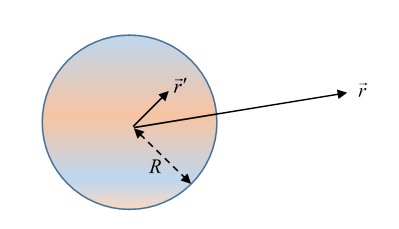
Consider the far away electric potential from a bounded charge distribution, say one confined to a sphere of radius $R.$  For $r\gg R,$ the potential will tend to $\left(1/4\pi {\epsilon }_0\right)Q/r,$ where $Q$ is the net charge, we’ll refer to this as the monopole potential.

If there is zero net charge, but the centroid of the positive charges (analogous to center of mass) differs from that of the negative charges, the distribution is said to have a dipole moment, and the dominant far potential will be that of a dipole.  

Any general charge distribution will generate a potential that is a sum of such terms: monopole, dipole, quadrupole, etc.

There are two common approaches to analyzing these moments:

● using $r,\theta ,\varphi$ coordinates and spherical harmonics,

● using $x,y,z$ and Cartesian moments.

Which of these to use depends to some extent on the problem at hand.  It is necessary to be familiar with both, and how they relate to each other.

We’ll first consider the spherical approach, then the Cartesian analysis.

Formal Expansion in Spherical Harmonics:  Multipole Moments

Suppose we have a distribution of charge $\rho \left({\overrightarrow{r}}^{\prime }\right),$ only nonzero for $r^{\prime }<R.$

The potential is

$$\phi \left(\overrightarrow{r}\right)=\frac{1}{4\pi {\epsilon }_0}{\displaystyle \underset{r\text{'}<R}{\int }\frac{\rho \left({\overrightarrow{r}}^{\prime }\right)}{\left|\overrightarrow{r}-{\overrightarrow{r}}^{\prime }\right|}{d}^3{r}^{\prime }}$$

and can be broken into moments at distances $\left|\overrightarrow{r}\right|>R$ by using the expansion (end of lecture 18)

$\frac{1}{\left|\overrightarrow{r}-\overrightarrow{R}\right|}={\displaystyle \sum _{l=0}^{\infty }\frac{r_{<}^l}{r_{>}^{l+1}}{P}_l\left(\cos \gamma \right)}=4\pi {\displaystyle \sum _{l=0}^{\infty }\frac{1}{2l+1}\frac{r_{<}^l}{r_{>}^{l+1}}{\displaystyle \sum _{m=-l}^l{Y}_l^m*\left({\theta }^{\prime },{\varphi }^{\prime }\right)Y_l^m\left(\theta ,\varphi \right)}}$

to get (putting $r_{<}=r^{\prime },r_{>}=r$ )

$\phi \left(\overrightarrow{r}\right)=\frac{1}{4\pi {\epsilon }_0}{\displaystyle \int \frac{\rho \left({\overrightarrow{r}}^{\prime }\right)}{\left|\overrightarrow{r}-{\overrightarrow{r}}^{\prime }\right|}{d}^3{r}^{\prime }}=\frac{1}{{\epsilon }_0}{\displaystyle \sum _{l=0}^{\infty }\frac{1}{2l+1}{\displaystyle \sum _{m=-l}^l\left[{\displaystyle \int Y_l^m*\left({\theta }^{\prime },{\varphi }^{\prime }\right){r^{\prime }}^l\rho \left({\overrightarrow{r}}^{\prime }\right)d^3{r}^{\prime }}\right]\frac{Y_l^m\left(\theta ,\varphi \right)}{r^{l+1}}}.}$

The multipole moments are defined as

$q_{lm}={\displaystyle \int Y_l^m*\left({\theta }^{\prime },{\varphi }^{\prime }\right){r^{\prime }}^l\rho \left({\overrightarrow{r}}^{\prime }\right)d^3{r}^{\prime }}$

so the potential outside the charge distribution can be expressed as a sum of multipole terms

$\phi \left(\overrightarrow{r}\right)=\frac{1}{{\epsilon }_0}{\displaystyle \sum _{l=0}^{\infty }\frac{1}{2l+1}{\displaystyle \sum _{m=-l}^l{q}_{lm}\frac{Y_l^m\left(\theta ,\varphi \right)}{r^{l+1}}}}.$

That is, each multipole moment of the charge distribution generates a potential field reflecting its own angular pattern:  don’t worry if you’re unfamiliar with these terms, we’ll discuss and illustrate in much more detail below.   

For convenience of reference (especially in connecting them with Cartesian moments in the following section) we’ll list here the first and second order spherical harmonics:

$Y_0^0=\frac{1}{\sqrt{4\pi }},Y_1^1=-\sqrt{\frac{3}{8\pi }}\sin \theta e^{i\varphi },Y_1^0=\sqrt{\frac{3}{4\pi }}\cos \theta ,Y_1^{-1}=\sqrt{\frac{3}{8\pi }}\sin \theta e^{-i\varphi }$

and

$\begin{array}{l}{Y}_2^2=\sqrt{\frac{15}{32\pi }}{\sin }^2\theta e^{2i\varphi },Y_2^1=-\sqrt{\frac{15}{8\pi }}\sin \theta \cos \theta e^{i\varphi },Y_2^0=\sqrt{\frac{5}{16\pi }}\left(3{\cos }^2\theta -1\right)\\ Y_2^{-2}=\sqrt{\frac{15}{32\pi }}{\sin }^2\theta e^{-2i\varphi },Y_2^{-1}=\sqrt{\frac{15}{8\pi }}\sin \theta \cos \theta e^{-i\varphi }.\end{array}$

Expressing Harmonics in Cartesian Coordinates

In fact, charge distributions are often given in Cartesian coordinates, so it's useful to express these $\left(\theta ,\varphi \right)$ multipole moments in Cartesian coordinates:

Using $\left(x,y,z\right)=\left(r\sin \theta \cos \varphi ,r\sin \theta \sin \varphi ,r\cos \theta \right)$ gives

$Y_1^1\left(x,y,z\right)=-\sqrt{\frac{3}{8\pi }}\cdot \frac{x+iy}{r},Y_1^0\left(x,y,z\right)=\sqrt{\frac{3}{4\pi }}\cdot \frac{z}{r},Y_1^{-1}\left(x,y,z\right)=\sqrt{\frac{3}{8\pi }}\cdot \frac{x-iy}{r}$

and

$Y_2^2=\sqrt{\frac{15}{32\pi }}\frac{{\left(x+iy\right)}^2}{r^2},Y_2^1=-\sqrt{\frac{15}{8\pi }}\frac{\left(x+iy\right)z}{r^2},Y_2^0=\sqrt{\frac{5}{16\pi }}\frac{\left(3z^2-1\right)}{r^2},\text{ etc}\text{.}$

Notice that in this representation, the $x,y$ coordinates only appear in the combinations $x\pm iy.$ 

This is easy to understand: the multipole moments are defined in terms of rotational eigenstates about the $z\text{-}$ axis, the spherical harmonics,  and the rotation operator is

$R_z\left(\theta \right)=\left(\begin{array}{ccc}\cos \theta & -\sin \theta & 0\\ \sin \theta & \cos \theta & 0\\ 0& 0& 1\end{array}\right),\text{with eigenvectors }\frac{1}{\sqrt{2}}\left(\begin{array}{c}1\\ i\\ 0\end{array}\right),\frac{1}{\sqrt{2}}\left(\begin{array}{c}1\\ -i\\ 0\end{array}\right),\left(\begin{array}{c}0\\ 0\\ 1\end{array}\right).$

The eigenvalues are $e^{\pm i\theta },1.$ 

(Mermin has argued in fact that the best coordinates for dealing with spherical harmonics are $\left(\xi ,\eta ,z\right)$ where $\xi =x+iy,\eta =x-iy.$ )

See the real spherical harmonics (with great visualization) here.

 Cartesian Moments Expansion

Very often the multipoles are conveniently expressed in terms of Cartesian moments.

Again, beginning with

$\phi \left(\overrightarrow{r}\right)=\frac{1}{4\pi {\epsilon }_0}{\displaystyle \int d^3{r}^{\prime }\frac{\rho \left({\overrightarrow{r}}^{\prime }\right)}{\left|\overrightarrow{r}-{\overrightarrow{r}}^{\prime }\right|}},$

for $r>r^{\prime },$ this time we make a Cartesian expansion:

$\frac{1}{\left|\overrightarrow{r}-{\overrightarrow{r}}^{\prime }\right|}=\frac{1}{r}-{\overrightarrow{r}}^{\prime }\cdot \overrightarrow{\nabla }\frac{1}{r}+\frac{1}{2}{\left({\overrightarrow{r}}^{\prime }\cdot \overrightarrow{\nabla }\right)}^2\frac{1}{r}-\cdots ,$

to get

$\phi \left(\overrightarrow{r}\right)=\frac{1}{4\pi {\epsilon }_0}\left\{\left[{\displaystyle \int d^3{r}^{\prime }\rho \left({\overrightarrow{r}}^{\prime }\right)}\right]\frac{1}{r}-\left[{\displaystyle \int d^3{r}^{\prime }\rho \left({\overrightarrow{r}}^{\prime }\right){r^{\prime }}_i}\right]{\nabla }_i\frac{1}{r}+\left[\frac{1}{2}{\displaystyle \int d^3{r}^{\prime }\rho \left({\overrightarrow{r}}^{\prime }\right){r^{\prime }}_i}{r^{\prime }}_j\right]{\nabla }_i{\nabla }_j\frac{1}{r}-\cdots \right\}$.

The expressions in square parentheses $\left[\right]$ are the Cartesian moments.

The Monopole

The total charge $Q={\displaystyle \int \rho \left({\overrightarrow{r}}^{\prime }\right)}{d}^3{r}^{\prime }$ is called the monopole moment in this notation. Notice that it contributes a term $Q/4\pi {\epsilon }_{0}r$ to the distant potential:  if it's nonzero, this is the leading term far enough away, and corresponds to replacing the charge distribution by a single point charge at the origin.  If the charge distribution is spherically symmetric, this is the only term in the $r>R$ expansion.

The Dipole

If the centroid of the positive charge (defined like center of mass) is not the same as that of the negative charge, the second term in the series for $\phi \left(\overrightarrow{r}\right)$ is nonzero.

This is the dipole moment, in the standard notation

$\overrightarrow{p}={\displaystyle \int {\overrightarrow{r}}^{\prime }}\rho \left({\overrightarrow{r}}^{\prime }\right)d^3{r}^{\prime }.$

The potential from the dipole moment term is

$-\frac{1}{4\pi {\epsilon }_0}\overrightarrow{p}\cdot \overrightarrow{\nabla }\left(\frac{1}{r}\right)=\frac{1}{4\pi {\epsilon }_0}\frac{\overrightarrow{p}\cdot \overrightarrow{r}}{r^3},$

and the electric field is

$\overrightarrow{E}\left(\overrightarrow{r}\right)=-\overrightarrow{\nabla }\phi \left(\overrightarrow{r}\right)=\frac{1}{4\pi {\epsilon }_0}\frac{3\widehat{\overrightarrow{r}}\left(\widehat{\overrightarrow{r}}\cdot \overrightarrow{p}\right)-\overrightarrow{p}}{r^3}.$

The (correctly normalized) spherical dipole moments in terms of the Cartesian moments are

$q_{11}=-\sqrt{\frac{3}{8\pi }}{\displaystyle \int \left(x^{\prime }-i{y}^{\prime }\right)\rho \left({\overrightarrow{r}}^{\prime }\right)d^3{r}^{\prime }}=-\sqrt{\frac{3}{8\pi }}\left(p_x-i{p}_y\right),q_{10}=\sqrt{\frac{3}{4\pi }}z,q_{1-1}=-q_{11}^{*}.$

Definition of a Point Dipole

The point dipole is a useful concept in discussing compact charge distributions in external fields that vary slowly over the extent of the charges.  (There is also the possibility that some elementary particles have nonzero electric dipole moments. This is currently under active investigation.) 

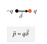
The point dipole is defined as the limit of two equal and opposite charges $\pm q$, separated by a small displacement $\overrightarrow{\delta },$ in the limit $\overrightarrow{\delta }\to 0$ under the condition that $q\overrightarrow{\delta }=\overrightarrow{p}$ is held constant.

The vector $\overrightarrow{p}$ is called the dipole moment, $\overrightarrow{\delta }$ points from the negative charge to the positive charge.

The potential from a dipole at the origin is

$\phi \left(\overrightarrow{r}\right)=\underset{\overrightarrow{\delta }\to 0}{\lim }\frac{1}{4\pi {\epsilon }_0}\left(\frac{q}{\left|\overrightarrow{r}-\overrightarrow{\delta }\right|}-\frac{q}{\left|\overrightarrow{r}\right|}\right)=-\frac{1}{4\pi {\epsilon }_0}q\overrightarrow{\delta }\cdot \overrightarrow{\nabla }\left(\frac{1}{r}\right)=\frac{1}{4\pi {\epsilon }_0}\frac{\overrightarrow{p}\cdot \overrightarrow{r}}{r^3}.$

Remark: the water molecule has a big electric dipole moment.  This is why water has a very large dielectric constant (although it goes way down at high frequencies, where the rotating molecule cannot fully respond).

Another Reciprocation Theorem: Charge and Field, Newton’s Third Law

Here's another trivial reciprocation theorem that turns out to be amazingly useful.

Suppose we have two charge distributions, A and B.  Distribution A has charge density ${\rho }_A\left(\overrightarrow{r}\right),$ this charge generates an electric field ${\overrightarrow{E}}_A\left(\overrightarrow{r}\right).$  Charge distribution B has density ${\rho }_B\left(\overrightarrow{r}\right)$ and field ${\overrightarrow{E}}_B\left(\overrightarrow{r}\right).$ 

What is the mutual force of interaction between these two charge distributions?  Clearly, it's

${\displaystyle \int {\rho }_A\left(\overrightarrow{r}\right){\overrightarrow{E}}_B\left(\overrightarrow{r}\right)}{d}^{3}r=-{\displaystyle \int {\rho }_B\left(\overrightarrow{r}\right){\overrightarrow{E}}_A\left(\overrightarrow{r}\right)}{d}^{3}r,$

the minus sign from Newton's third law.  This is our reciprocation theorem!

Exercise:  check by appropriate differentiation that this reciprocation theorem follows from Green's original one, about potentials and charges.

Electric Dipole: Some Useful Insights from the Reciprocation Theorem

Theorem:  For a charge distribution completely contained in a sphere of radius $R,$ the net dipole moment of the distribution is proportional to the average value of the electric field inside the sphere.

$${\displaystyle \underset{V}{\int }\overrightarrow{E}}{d}^{3}r=-\frac{{\overrightarrow{p}}_{\text{tot}}}{3{\epsilon }_0}.$$

Think reciprocation theorem (previous section).

Calling the electric field ${\overrightarrow{E}}_A\left(\overrightarrow{r}\right)$ from a charge distribution ${\rho }_A\left(\overrightarrow{r}\right),$ what charge distribution ${\rho }_B\left(\overrightarrow{r}\right)$ will give me the left-hand side of the above equation?

Evidently, a charge density equal to one in the relevant volume:

${\rho }_B\left(\overrightarrow{r}\right)=1,r\le R;{\rho }_B\left(\overrightarrow{r}\right)=0,r>R.$

Then, from Gauss' theorem, the (spherically symmetric) electric field ${\overrightarrow{E}}_B\left(\overrightarrow{r}\right)$  from this ${\rho }_B\left(\overrightarrow{r}\right)$ given by $4\pi r^{2}E=\left(4/3\right)\pi r^3/{\epsilon }_0$, that is, inside the sphere the electric field (analogous to the gravitational field inside a uniform Earth)

$${\overrightarrow{E}}_B\left(\overrightarrow{r}\right)=\frac{\overrightarrow{r}}{3{\epsilon }_0},r\le R.$$

The total electric force from this field on ${\rho }_A\left(\overrightarrow{r}\right)$ (which is all within the sphere) is

$${\displaystyle \underset{V}{\int }{\rho }_A\left(\overrightarrow{r}\right)}{\overrightarrow{E}}_B\left(\overrightarrow{r}\right)d^{3}r=\frac{1}{3{\epsilon }_0}{\displaystyle \underset{V}{\int }{\rho }_A\left(\overrightarrow{r}\right)}\overrightarrow{r}{d}^{3}r=\frac{{\overrightarrow{p}}_A}{3{\epsilon }_0},$$

from the definition of the dipole moment of a charge distribution.

But this force must be equal and opposite to the force on the sphere from the electric field of the charge distribution, which is (remember ${\rho }_B\left(\overrightarrow{r}\right)=1$ within the sphere):

${\displaystyle \underset{V}{\int }{\rho }_A\left(\overrightarrow{r}\right)}{\overrightarrow{E}}_B\left(\overrightarrow{r}\right)d^{3}r=-{\displaystyle \underset{V}{\int }{\overrightarrow{E}}_B\left(\overrightarrow{r}\right)d^{3}r}.$

The result follows:

$${\displaystyle \underset{V}{\int }{\overrightarrow{E}}_A\left(\overrightarrow{r}\right)}{d}^{3}r=-\frac{{\overrightarrow{p}}_A}{3{\epsilon }_0}.$$

Average Electric Field in a Charge-Free Spherical Volume

What about a charge distribution completely outside some spherical volume?  It turns out that in this case, the average value of the electric field in the sphere is exactly its value at the center of the sphere:

${\displaystyle \underset{r<R}{\int }\overrightarrow{E}\left(\overrightarrow{r}\right)d^{3}r}=\frac{4}{3}\pi R^3\overrightarrow{E}\left(0\right),$

taking the sphere to be centered at the origin.

To prove this, imagine inserting a sphere of radius $R$ having unit charge density throughout, and assume all the other charges are frozen in place as this happens. Then the force on the charged sphere from the other charges is just the integral on the left-hand side of the equation.  But since the inserted sphere does not overlap the preexisting charge distribution, those other charges experience forces identical to those from a point charge at the origin. Therefore, they must exert a force on our sphere equal to the force they would exert on a point charge at the origin equal to the charge of the whole sphere. Since the charge density is unity, the total charge is just the volume of the sphere, that is, the right-hand side of the above equation.

For a general charge distribution, inside and outside the sphere, the average of the electric field throughout a sphere is evidently a sum of the two terms found above.  

A Dipole Field Puzzle

Now let’s look at the field from a point dipole at the origin. (Although there's no evidence a true point dipole exists in the Universe.)

We know from the theorem in the previous section that (taking the spherical volume to infinity)

$${\displaystyle \underset{V}{\int }\overrightarrow{E}\left(\overrightarrow{r}\right)d^{3}r}=-\frac{1}{3{\epsilon }_0}{\displaystyle \underset{r^{\prime }<R}{\int }\rho \left({\overrightarrow{r}}^{\prime }\right){\overrightarrow{r}}^{\prime }}{d}^3{r}^{\prime }=-\frac{\overrightarrow{p}}{3{\epsilon }_0}.$$

Now recall what the field from a dipole looks like:

$$\overrightarrow{E}\left(\overrightarrow{r}\right)=\frac{1}{4\pi {\epsilon }_0}\frac{3\widehat{\overrightarrow{r}}\left(\widehat{\overrightarrow{r}}\cdot \overrightarrow{p}\right)-\overrightarrow{p}}{r^3}.$$

If we integrate this over space, since it's axially symmetric, the resultant vector (if any) has to be in the $\overrightarrow{p}$ direction.  But

${\displaystyle \int \overrightarrow{E}\cdot \overrightarrow{p}{d}^{3}r}={\displaystyle \int \frac{d^{3}r}{4\pi {\epsilon }_0}\frac{3{\left(\widehat{\overrightarrow{r}}\cdot \overrightarrow{p}\right)}^2-{\overrightarrow{p}}^2}{r^3}}={\displaystyle \int \frac{d^{3}r}{4\pi {\epsilon }_0}\frac{p^2\left(3{\cos }^2\theta -1\right)}{r^3}=0,}$

seemingly contradicting our theorem!

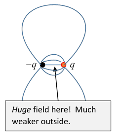
The point is that an electric dipole isn't actually at a mathematical point:  it's two large opposite charges very close together, so there is a very large field between them, which we’ve ignored in constructing the dipole field, but we can’t ignore if we’re really going to integrate the electric field over all space.  

Let’s just check the order of magnitude of that inside-the-dipole contribution: suppose the dipole is two charges $\pm q$ a distance $d$ apart, so $p=qd.$ Then in between the charges, the field is of strength $\sim q/d^2$ over a volume $\sim d^3$, so the integral over this tiny region will give a contribution $\sim qd=p$.  Of course, we don’t need to evaluate the integral, our argument above will be valid in the limit of constructing a dipole by moving charges together and increasing their magnitude at the same time, so the electric field at $\overrightarrow{r}$ from a dipole at the origin is

$$\overrightarrow{E}\left(\overrightarrow{r}\right)=\frac{1}{4\pi {\epsilon }_0}\left[\frac{3\widehat{\overrightarrow{r}}\left(\overrightarrow{p}\cdot \widehat{\overrightarrow{r}}\right)-\overrightarrow{p}}{r^3}-\frac{4\pi }{3}\overrightarrow{p}\delta \left(\overrightarrow{r}\right)\right].$$

Force on a Dipole in an Electric Field

For a constant field, there is no net force on a dipole, since the two charges are opposite.  But there will be a torque: take the dipole to be two charges $\pm q$ separated by distance $\overrightarrow{\delta }$ (pointing towards the positive charge) and the field $\overrightarrow{E}.$  Writing $\overrightarrow{p}=q\overrightarrow{\delta },$ the torque $\overrightarrow{N}=\overrightarrow{p}\times \overrightarrow{E}.$  

If the field is nonuniform, then there will also be a net force, equal to that on the positive charge minus that on the negative charge,

$$\overrightarrow{F}=q\overrightarrow{E}\left(\overrightarrow{r}+\frac{1}{2}\overrightarrow{\delta }\right)-q\overrightarrow{E}\left(\overrightarrow{r}-\frac{1}{2}\overrightarrow{\delta }\right)=\overrightarrow{p}\cdot \overrightarrow{\nabla }\overrightarrow{E}.$$

The dipole potential energy from the torque is easily seen to be $-\overrightarrow{p}\cdot \overrightarrow{E}.$  Just visualize where the two charges are in the electric potential.

The dipole-dipole interaction energy is found by differentiating the potential of a dipole in the direction of a second dipole. That is, it's $\frac{1}{4\pi {\epsilon }_0}\left({\overrightarrow{p}}_1\cdot \overrightarrow{\nabla }\right)\left({\overrightarrow{p}}_2\cdot \overrightarrow{\nabla }\right)\frac{1}{r}$ ,

$$W_{12}=\frac{1}{4\pi {\epsilon }_0}\left\{\frac{{\overrightarrow{p}}_1\cdot {\overrightarrow{p}}_2}{r^3}-\frac{\left({\overrightarrow{p}}_1\cdot \overrightarrow{r}\right)\left({\overrightarrow{p}}_2\cdot \overrightarrow{r}\right)}{r^5}\right\}.$$

The Quadrupole Moment

Recall now the expansion of the electric potential from a localized charge distribution:

$$\begin{array}{c}\phi \left(\overrightarrow{r}\right)=\frac{1}{4\pi {\epsilon }_0}\left\{\left[{\displaystyle \int d^3{r}^{\prime }\rho \left({\overrightarrow{r}}^{\prime }\right)}\right]\frac{1}{r}-\left[{\displaystyle \int d^3{r}^{\prime }\rho \left({\overrightarrow{r}}^{\prime }\right){r^{\prime }}_i}\right]{\nabla }_i\frac{1}{r}+\left[\frac{1}{2}{\displaystyle \int d^3{r}^{\prime }\rho \left({\overrightarrow{r}}^{\prime }\right){r^{\prime }}_i}{r^{\prime }}_j\right]{\nabla }_i{\nabla }_j\frac{1}{r}-\cdots \right\}\\ =\frac{1}{4\pi {\epsilon }_0}\left\{\frac{Q}{r}+\frac{\overrightarrow{p}\cdot \overrightarrow{r}}{r^3}+\left[\frac{1}{2}{\displaystyle \int d^3{r}^{\prime }\rho \left({\overrightarrow{r}}^{\prime }\right){r^{\prime }}_i}{r^{\prime }}_j\right]\frac{3r_i{r}_j-r^2{\delta }_{ij}}{r^5}\cdots \right\}\end{array}$$

The third term is the quadrupole contribution to the potential from the charge distribution.  The term in square brackets is the quadrupole moment tensor, symmetric and 3x3, so apparently having six independent elements. However, the standard procedure is to rearrange in a simple way to make manifest that in fact we can choose a traceless quadrupole tensor without loss of information, so actually there are only five independent parameters in the quadrupole.

We rearrange as follows:

$$\frac{3r_i{r}_j-r^2{\delta }_{ij}}{r^5}{\displaystyle \int d^3{r}^{\prime }\rho \left({\overrightarrow{r}}^{\prime }\right)}{r}_i{}^{\prime }{r}_j{}^{\prime }=\frac{r_i{r}_j}{r^5}{\displaystyle \int d^3{r}^{\prime }\rho \left({\overrightarrow{r}}^{\prime }\right)}\left(3r_i{}^{\prime }{r}_j{}^{\prime }-{\delta }_{ij}{r^{\prime }}^2\right),$$

using $r^2{\delta }_{ij}{r}_i{}^{\prime }{r}_j{}^{\prime }=r^2{r^{\prime }}^2={r^{\prime }}^2{\delta }_{ij}{r}_i{r}_j,$ and define the (traceless) quadrupole moment by

$$Q_{ij}={\displaystyle \int d^{3}r\rho \left(\overrightarrow{r}\right)}\left(3r_i{r}_j-r^2{\delta }_{ij}\right)=Q_{ji},$$

${\phi }_{\text{quad}}\left(\overrightarrow{r}\right)=\frac{1}{4\pi {\epsilon }_0}\cdot \frac{1}{2}\cdot Q_{ij}\frac{r_i{r}_j}{r^5}.$

(As usual, primed variables denote positions of charges, unprimed the point outside where we're finding the potential.)

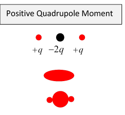
Just as a dipole can be thought of as two equal magnitude opposite sign charges slightly displaced, a quadrupole can be thought of as two equal but opposite dipoles slightly displaced. 

In general, this displacement won't be along the line of the dipoles, so the potential can be represented as

$$\phi \left(\overrightarrow{r}\right)=\frac{1}{4\pi {\epsilon }_0}\left(\overrightarrow{c}\cdot \overrightarrow{\nabla }\right)\left(\overrightarrow{p}\cdot \overrightarrow{\nabla }\right)\frac{1}{r}.$$

This agrees with the expression above (symmetric in $i,j$ )  if

$Q_{ij}=\frac{1}{2}\left(c_i{p}_j+p_i{c}_j\right).$

An important quadrupole moment of practical use is that of a nucleus.  Most nuclei are not spherical, but spheroidal, with one axis of rotational symmetry. It's reasonable to assume, at least to begin with, that the electric charge is uniformly distributed throughout the ellipsoidal volume.  Clearly there is zero dipole moment, but for non-spherical nuclei, there is a nonzero quadrupole moment, for example,

$Q_{zz}=\frac{1}{2}{\displaystyle \int d^3{r}^{\prime }\rho \left({\overrightarrow{r}}^{\prime }\right)}\left(3{z^{\prime }}^2-{r^{\prime }}^2\right)=\frac{1}{2}{\displaystyle \int d^3{r}^{\prime }\rho \left({\overrightarrow{r}}^{\prime }\right)}\left(2{z^{\prime }}^2-{x^{\prime }}^2-{y^{\prime }}^2\right),$

The integration being over the ellipsoidal volume $\frac{{x^{\prime }}^2+{y^{\prime }}^2}{a^2}+\frac{{z^{\prime }}^2}{c^2}=1.$  This is a difficult integral as it stands, because of the difficult boundary requirement, but the remedy is simple: scale the ellipsoid to a sphere.  That is, change variables to $x=x^{\prime }/a,y=y^{\prime }/a,z=z^{\prime }/c.$ 

The integral becomes

$Q_{zz}=\frac{1}{2}{a}^{2}c\rho {\displaystyle \underset{r\le 1}{\int }dxdydz\left(2c^2{z}^2-a^2{x}^2-a^2{y}^2\right)}.$

Now ${\displaystyle \underset{r\le 1}{\int }dxdydz{z}^2}=\frac{1}{3}{\displaystyle \underset{r\le 1}{\int }dxdydz{r}^2}=\frac{4\pi }{3}{\displaystyle \underset{r\le 1}{\int }{r}^2{r}^{2}dr}=\frac{4\pi }{15},$    from which (using the volume of the ellipsoid $V=\frac{4}{3}\pi a^{2}c$ ) we have

$Q_{zz}=\frac{1}{5}\rho V\left(c^2-a^2\right).$

Nuclear Quadrupole Moments

Almost all nuclei are spheroidal, so the only relevant quadrupole moment is $Q_{zz}$ given above. The other two diagonal elements are equal, and tracelessness ensures they are each $-\frac{1}{2}{Q}_{zz}.$  Off diagonal elements are zero by symmetry.

The moment has dimensions charge x area, widely used units are e.b where e is the electron charge, b is the barn,  b = 10^-28 m².  (This name was coined by classified researchers on nuclear bombs who wanted a term that would be difficult to understand by spies. It is about the cross-section of a uranium nucleus, so should be easy to hit: hence, the barn door.  A smaller target, the microbarn, is called the outhouse.

Most nuclei have positive quadrupole moments, meaning they are prolate spheroids, but some have negative moments, meaning they are oblate.  To see why a prolate spheroid has positive quadrupole moment, imagine it as a sphere (which has zero quadrupole moment) with extra positive charge added to the north and south poles.  (And, for good measure, you could scrape a belt of positive charge off the equator).

Why do nuclei have quadrupole moments anyway? The dominant interaction holding the nucleons together is the strong force, an early model was the liquid drop model, fairly successful in predicting binding energies, but it doesn't suggest why the drop apparently isn't spherical in most cases.

Some enlightenment came with the realization that the shell model, somewhat like the electron shells in an atom, might be partially correct. Sure enough, it turned out that for light nuclei, there were "magic numbers", starting with helium, corresponding to particularly strong binding.  The atomic analogy has its limitations, though, because within the nucleus spin-orbit coupling is far stronger than for atomic electrons, especially for heavier nuclei, so angular momentum and spin are no longer good separate quantum numbers for the nucleons. We won't pursue this further here, suffice to say that there is clearly some validity to the shell picture, so it's easy to imagine that a closed shell plus a couple more nucleons won't be a perfect sphere. 

Interaction of a Quadrupole with an External Electric Field

 Just as a dipole, two opposite charges a small distance apart, lines up with the electric field, a quadrupole, two opposite dipoles a small distance apart, aligns along the direction of the field gradient. For our case of spheroidal nuclei, then, the axis of symmetry lines up along the field gradient.

Imagine a compact charge distribution in a region around the origin, and a reasonably slowly varying (in position) electric field. The energy of the charge distribution in this field can then be expanded in moments:

$\begin{array}{c}U={\displaystyle \int \rho \left(\overrightarrow{r}\right)\phi \left(\overrightarrow{r}\right)}{d}^{3}r\\ ={\displaystyle \int {\displaystyle \int \rho \left(\overrightarrow{r}\right)\left[\phi \left(0\right)+\overrightarrow{r}\cdot \overrightarrow{\nabla }\phi \left(0\right)+\frac{1}{2}{{\displaystyle \sum _{i,j}{r}_i{r}_j\left.\frac{{\partial }^2\phi }{\partial r_i\partial r_j}\right|}}_{r=0}+\cdots \right]}{d}^{3}r}\\ =QV\left(0\right)-\overrightarrow{p}\cdot \overrightarrow{E}\left(0\right)-\frac{1}{6}{\displaystyle \sum _{i,j}\left[{\displaystyle \int d^{3}r\rho \left(\overrightarrow{r}\right)\left(3r_i{r}_j-r^2{\delta }_{ij}\right){\left.\frac{\partial E_j}{\partial r_i}\right|}_{r=0}+\cdots }\right]}\\ =QV\left(0\right)-\overrightarrow{p}\cdot \overrightarrow{E}\left(0\right)-\frac{1}{6}{\displaystyle \sum _{i,j}{Q}_{ij}{\left.\frac{\partial E_j}{\partial r_i}\right|}_{r=0}+\cdots }\end{array}$

where we've used $\overrightarrow{\nabla }\cdot \overrightarrow{E}=0$ for the external field.

For the particular case of the spheroidal nucleus, the last term becomes

$$-\frac{1}{6}\left[Q_{zz}\frac{\partial E_z}{\partial z}+Q_{xx}\frac{\partial E_x}{\partial x}+Q_{yy}\frac{\partial E_y}{\partial y}\right]$$

And, with $Q_{xx}=Q_{yy}=-\frac{1}{2}{Q}_{zz},$ and $\overrightarrow{\nabla }\cdot \overrightarrow{E}=0,$ we can finally write the quadrupole interaction energy as

$$U_{\text{quadrupole}}=-\frac{1}{3}{Q}_{zz}\frac{\partial E_z}{\partial z}.$$

Nuclear Quadrupole Resonance

A spin one nucleus can have $m=1,0,-1$ with respect to a given direction.  If it has a nuclear quadrupole moment, and is in an electric field of varying strength, its lowest energy state will be in alignment with the gradient of the field (but pointing either way.)  For spin one, there are two different energy levels, $m=0,m=\pm 1.$

Luckily, the nitrogen nucleus has a quadrupole moment, and spin one.  The electric field at a nucleus depends on the nitrogen nucleus’ positioning in a molecule, so different chemicals have different energy splitting of the quadrupole states.  The order of magnitude of the energy level difference is that of megahertz photons, so these can readily be detected by looking for a response of the substance to a megahertz signal (amplified by spin echo techniques).

Since almost all explosives contain nitrogen, and the resonance response spectrum is well defined, making them easy to differentiate, and distinguish from other nitrogen-bearing materials, this would seem ideal for bomb detection, and this has been argued.  However, it does not seem to be in wide use currently, possibly because a fake device (ADE 651), produced in the UK, supposedly based on NQR, was sold for millions of dollars to various governments.  Also, it’s really easy to shield against microwaves.

previous  index  next