previous  index  next 

31.  Magnetostatics II: Vector Potential, Field from Localized Currents, Scalar Potential

    Michael Fowler, UVa

Vector Potential

From the previous lecture the Maxwell equations for magnetostatics are:

$$\begin{array}{c}\overrightarrow{\nabla }\cdot \overrightarrow{B}\left(\overrightarrow{r}\right)=0,\\ \overrightarrow{\nabla }\times \overrightarrow{B}\left(\overrightarrow{r}\right)={\mu }_0\overrightarrow{j}\left(\overrightarrow{r}\right).\end{array}$$

Putting these into Helmholtz’ equation for $\overrightarrow{B}\left(\overrightarrow{r}\right)$ gives

$$\overrightarrow{B}\left(\overrightarrow{r}\right)=\overrightarrow{\nabla }\times \frac{{\mu }_0}{4\pi }{\displaystyle \int d^3{r}^{\prime }}\frac{\overrightarrow{j}\left({\overrightarrow{r}}^{\prime }\right)}{\left|\overrightarrow{r}-{\overrightarrow{r}}^{\prime }\right|},$$

expressing the magnetic field as the curl of a vector potential $\overrightarrow{A}\left(\overrightarrow{r}\right)$:        

$$\begin{array}{l}\overrightarrow{B}\left(\overrightarrow{r}\right)=\overrightarrow{\nabla }\times \overrightarrow{A}\left(\overrightarrow{r}\right),\\ \overrightarrow{A}\left(\overrightarrow{r}\right)=\frac{{\mu }_0}{4\pi }{\displaystyle \int d^3{r}^{\prime }}\frac{\overrightarrow{j}\left({\overrightarrow{r}}^{\prime }\right)}{\left|\overrightarrow{r}-{\overrightarrow{r}}^{\prime }\right|}.\end{array}$$

Notice that the dependence of this vector potential on the current distribution is exactly parallel to the dependence of the electrostatic (scalar) potential on the charge distribution:

$$\phi \left(\overrightarrow{r}\right)=\frac{1}{4\pi {\epsilon }_0}{\displaystyle \int d^3{r}^{\prime }}\frac{\rho \left({\overrightarrow{r}}^{\prime }\right)}{\left|\overrightarrow{r}-{\overrightarrow{r}}^{\prime }\right|}.$$

Note: This will all become clearer when we get to relativity: $\left(\phi ,\overrightarrow{A}\right)$ and $\left(\rho ,\overrightarrow{j}\right)$ both transform as 4-vectors under the Lorentz group.

Magnetic Field of a Localized Current Distribution, Magnetic Moment

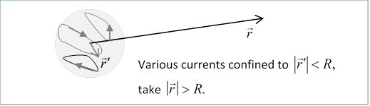
We’ll now consider the magnetic field generated by a steady current distribution confined to some region of space, and how it looks from some distance away. In other words, we’ll look at a multipole analysis of the magnetic field at a point $\overrightarrow{r}$ outside the region of current.

 

As usual, we use the expansion

$$\frac{1}{\left|\overrightarrow{r}-{\overrightarrow{r}}^{\prime }\right|}=\frac{1}{\left|\overrightarrow{r}\right|}+\frac{\overrightarrow{r}\cdot {\overrightarrow{r}}^{\prime }}{{\left|\overrightarrow{r}\right|}^3}+\cdots$$

to get for the $i$-component of the vector potential

$$A_i\left(\overrightarrow{r}\right)=\frac{{\mu }_0}{4\pi }\left[\frac{1}{\left|\overrightarrow{r}\right|}{\displaystyle \int j_i\left({\overrightarrow{r}}^{\prime }\right)d^3{r}^{\prime }}+\frac{\overrightarrow{r}}{{\left|\overrightarrow{r}\right|}^3}\cdot {\displaystyle \int {\overrightarrow{r}}^{\prime }{j}_i\left({\overrightarrow{r}}^{\prime }\right)d^3{r}^{\prime }}+\cdots \right].$$

Monopole Term

This first term in the series turns out to zero for a localized steady current distribution.

The standard proof is as follows: taking one component, and using, for example, $\overrightarrow{\nabla }x=\left(1,0,0\right)$,

${\displaystyle \int j_i{d}^3{r}^{\prime }}={\displaystyle \int \overrightarrow{j}\cdot {\overrightarrow{\nabla }}^{\prime }{r^{\prime }}_i{d}^3{r}^{\prime }}=-{\displaystyle \int {r^{\prime }}_i\left({\overrightarrow{\nabla }}^{\prime }\cdot \overrightarrow{j}\left({\overrightarrow{r}}^{\prime }\right)\right)d^3{r}^{\prime }}+{\displaystyle \int {\overrightarrow{\nabla }}^{\prime }\cdot \left({r^{\prime }}_i\overrightarrow{j}\left({\overrightarrow{r}}^{\prime }\right)\right)d^3{r}^{\prime }}$.

Since ${\overrightarrow{\nabla }}^{\prime }\cdot \overrightarrow{j}\left({\overrightarrow{r}}^{\prime }\right)=0,$ the first term on the right vanishes, and the second is a divergence, so the divergence theorem gives it as equal to an integral over the surface at infinity, where the current distribution (which we stated was confined to a finite region) will be zero. 

Or, you could just say that in a steady state, at any instant of time, the total current flow to the right must equal that to the left, or it won’t stay a steady state.

Dipole Term

The dipole term is:

$$A_i\left(\overrightarrow{r}\right)=\frac{{\mu }_0}{4\pi }\frac{\overrightarrow{r}}{{\left|\overrightarrow{r}\right|}^3}\cdot {\displaystyle \int {\overrightarrow{r}}^{\prime }{j}_i\left({\overrightarrow{r}}^{\prime }\right)d^3{r}^{\prime }},$$

This expression is not very illuminating, however.  We know, for example, that magnetic dipoles come from current loops, not straight lines of current, so we would naïvely expect to see electric current “angular momentum” terms, like ${\overrightarrow{r}}^{\prime }\times {\overrightarrow{j}}^{\prime }$ playing a role. It turns out (with hindsight, of course) that we can manipulate the above integral into a more understandable form with a few math tricks. Essentially, we need to introduce some antisymmetry into the integrand to get a cross-product coming out.

To do that, we find that we need to prove this lemma:

${\displaystyle \int {r^{\prime }}_j{j}_i\left({\overrightarrow{r}}^{\prime }\right)d^3{r}^{\prime }}=-{\displaystyle \int {r^{\prime }}_i{j}_j\left({\overrightarrow{r}}^{\prime }\right)d^3{r}^{\prime }}.$

In fact the result follows from conservation of current$—$plus the following identity (custom-made for the occasion):

$\begin{array}{c}{\overrightarrow{\nabla }}^{\prime }\cdot \left({r^{\prime }}_i{r^{\prime }}_j\overrightarrow{j}\left({\overrightarrow{r}}^{\prime }\right)\right)={r^{\prime }}_i{r^{\prime }}_j{\overrightarrow{\nabla }}^{\prime }\cdot \overrightarrow{j}\left({\overrightarrow{r}}^{\prime }\right)+{r^{\prime }}_j\left({\overrightarrow{\nabla }}^{\prime }{r^{\prime }}_i\right)\cdot \overrightarrow{j}\left({\overrightarrow{r}}^{\prime }\right)+{r^{\prime }}_i\left({\overrightarrow{\nabla }}^{\prime }{r^{\prime }}_j\right)\cdot \overrightarrow{j}\left({\overrightarrow{r}}^{\prime }\right)\\ =0+{r^{\prime }}_j{j}_i\left({\overrightarrow{r}}^{\prime }\right)+{r^{\prime }}_i{j}_j\left({\overrightarrow{r}}^{\prime }\right),\end{array}$

where we used, for example, $\overrightarrow{\nabla }x=\left(1,0,0\right).$

On integrating the identity over all space, the left-hand side gives zero, since the currents are in a bounded volume (and using Gauss’ theorem this equals a surface integral at infinity), establishing the lemma.    

Applying the lemma result to the expression for $A_i\left(\overrightarrow{r}\right)$  the dipole integral $\overrightarrow{r}\cdot {\displaystyle \int {\overrightarrow{r}}^{\prime }{j}_i\left({\overrightarrow{r}}^{\prime }\right)d^3{r}^{\prime }}$ can be rewritten:

$\begin{array}{c}{r}_j{\displaystyle \int j_i\left({\overrightarrow{r}}^{\prime }\right){r^{\prime }}_j{d}^3{r}^{\prime }}=\frac{1}{2}{r}_j{\displaystyle \int \left(j_i\left({\overrightarrow{r}}^{\prime }\right){r^{\prime }}_j-j_j\left({\overrightarrow{r}}^{\prime }\right){r^{\prime }}_i\right)d^3{r}^{\prime }}\\ =\frac{1}{2}{{\displaystyle \int \left[\overrightarrow{j}\left({\overrightarrow{r}}^{\prime }\right)\left(\overrightarrow{r}\cdot {\overrightarrow{r}}^{\prime }\right)-{\overrightarrow{r}}^{\prime }\left(\overrightarrow{r}\cdot \overrightarrow{j}\left({\overrightarrow{r}}^{\prime }\right)\right)\right]}}_i{d}^3{r}^{\prime }\\ =\frac{1}{2}{{\displaystyle \int \left[\left({\overrightarrow{r}}^{\prime }\times \overrightarrow{j}\left({\overrightarrow{r}}^{\prime }\right)\right)\times \overrightarrow{r}\right]}}_i{d}^3{r}^{\prime }.\end{array}$

At this point, we define the magnetic dipole moment of the current distribution as

$$\overrightarrow{m}=\frac{1}{2}{\displaystyle \int {\overrightarrow{r}}^{\prime }\times \overrightarrow{j}\left({\overrightarrow{r}}^{\prime }\right)}{d}^3{r}^{\prime },$$

so the dipole contribution to the vector potential is

$$\overrightarrow{A}\left(\overrightarrow{r}\right)=\frac{{\mu }_0}{4\pi }\frac{\overrightarrow{m}\times \overrightarrow{r}}{{\left|\overrightarrow{r}\right|}^3},$$

and the dipole magnetic field is:

$\begin{array}{c}\overrightarrow{B}\left(\overrightarrow{r}\right)=\overrightarrow{\nabla }\times \overrightarrow{A}\left(\overrightarrow{r}\right)\\ =\frac{{\mu }_0}{4\pi }\overrightarrow{\nabla }\times \frac{\overrightarrow{m}\times \overrightarrow{r}}{{\left|\overrightarrow{r}\right|}^3}\\ =\frac{{\mu }_0}{4\pi }\left[\overrightarrow{m}\left(\overrightarrow{\nabla }\cdot \frac{\overrightarrow{r}}{r^3}\right)-\overrightarrow{m}\cdot \overrightarrow{\nabla }\left(\frac{\overrightarrow{r}}{r^3}\right)\right]\\ =\frac{{\mu }_0}{4\pi }\left[\frac{3\widehat{\overrightarrow{r}}\left(\widehat{\overrightarrow{r}}\cdot \overrightarrow{m}\right)-\overrightarrow{m}}{{\left|\overrightarrow{r}\right|}^3}\right].\end{array}$

This is the exact same form as the electric dipole field, thus proving that our definition of the dipole moment of the currents was correct.

(Note:  We dropped that first term in going to the last line.  It’s just a delta function at the origin, and, remember, this expansion of the field in terms of moments is only valid at distances greater that the radius of the volume containing the currents, hence far from the origin.)

Quadrupole, etc.

For our present purposes, we do not need to investigate further terms in the multipole expansion, but we will need them later, for example when we investigate radiation from oscillating circuits.

Planar Current Loop

Suppose a current $I$ is flowing around some circuit in a plane. Taking the origin in the plane, inside the loop (for simplicity$—$this is not necessary) then

$\overrightarrow{m}=\frac{1}{2}{\displaystyle \int {\overrightarrow{r}}^{\prime }\times \overrightarrow{j}\left({\overrightarrow{r}}^{\prime }\right)}{d}^3{r}^{\prime }=\frac{1}{2}{\displaystyle \oint {\overrightarrow{r}}^{\prime }\times Id\overrightarrow{l}}=I\cdot \left(\text{Area}\right),$

and the $\overrightarrow{m}$ vector is perpendicular to the plane.

Exercise:  check that the origin could be outside the loop, and even out of the plane, and the result would be the same.

Note that if we view an electron in a circular orbit in an atom as classical, and replace it by an average current, the formula for the magnetic moment generated by the orbital motion has the same mathematical form as the orbital angular momentum, and in fact it’s easy to check that $\overrightarrow{m}=\left(e/m\right)\overrightarrow{L},$  so the mass is simply replaced by the charge. Remarkably, this formula is still good in quantum mechanics for orbital angular momentum, although off by a factor of 2 for the truly quantum-mechanical spin angular momentum.

Magnetic Scalar Potential

We can always represent a magnetic potential as the curl of a vector potential, but sometimes it can also be written as the gradient of a scalar potential, 

$$\overrightarrow{B}\left(\overrightarrow{r}\right)=-{\mu }_0\overrightarrow{\nabla }{\phi }_M\left(\overrightarrow{r}\right).$$

This scalar potential turns out to be useful in understanding magnetic materials, as we shall see a bit later, but it’s also helpful in finding the field from a current loop.

We showed in the previous lecture that (apart from the delta function at the origin) the magnetic dipole field is identical in form to the electric dipole field.

We showed in the second lecture that the electric dipole field can be written as the gradient of a potential,

$$\overrightarrow{E}\left(\overrightarrow{r}\right)=-\overrightarrow{\nabla }\phi \left(\overrightarrow{r}\right)=\frac{1}{4\pi {\epsilon }_0}\frac{3\widehat{\overrightarrow{r}}\left(\widehat{\overrightarrow{r}}\cdot \overrightarrow{p}\right)-\overrightarrow{p}}{r^3},$$

where

$$\phi \left(\overrightarrow{r}\right)=\frac{1}{4\pi {\epsilon }_0}\frac{\overrightarrow{p}\cdot \overrightarrow{r}}{r^3}.$$

Clearly the magnetic dipole field

$$\overrightarrow{B}\left(\overrightarrow{r}\right)=\overrightarrow{\nabla }\times \overrightarrow{A}\left(\overrightarrow{r}\right)=\frac{{\mu }_0}{4\pi }\frac{3\widehat{\overrightarrow{r}}\left(\widehat{\overrightarrow{r}}\cdot \overrightarrow{m}\right)-\overrightarrow{m}}{{\left|\overrightarrow{r}\right|}^3}$$

can be similarly expressed as the gradient of the scalar potential

$${\phi }_M\left(\overrightarrow{r}\right)=\frac{{\mu }_0}{4\pi }\frac{\overrightarrow{m}\cdot \overrightarrow{r}}{r^3}.$$

Now consider the magnetic field from a small planar current loop, as discussed in the previous section. The dipole moment

$$\overrightarrow{m}=I\Delta \overrightarrow{A},$$

where $\Delta \overrightarrow{A}$ is a vector with magnitude equal to the small area $\Delta A$ and direction, using the right-hand rule, perpendicular to the plane.

So  

$${\phi }_M\left(\overrightarrow{r}\right)=\frac{{\mu }_0}{4\pi }\frac{I\Delta \overrightarrow{A}\cdot \overrightarrow{r}}{r^3}=\frac{{\mu }_0}{4\pi }I\Delta \Omega ,$$

where $\Delta \Omega$ is the solid angle subtended by the small loop at the point $\overrightarrow{r}.$

Exercise:  Verify this.

 

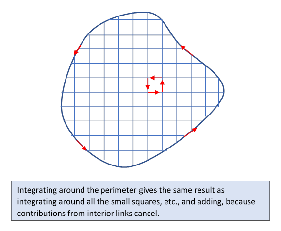
Suppose we now have a normal-sized current loop. By analogy with the usual proof of Stokes’ theorem, we can replace it with a network of tiny current loops, as in the diagram. The current $I$ goes around each small square (and around the irregularly shaped edge areas). Currents on all internal edges cancel, so the magnetic potential from the current around the outside loop is identical to that from the sum of all the small dipoles, that is,

$${\phi }_M\left(\overrightarrow{r}\right)=\frac{{\mu }_0}{4\pi }I\Omega ,$$

where $\Omega$ is the solid angle subtended at $\overrightarrow{r}$ by the whole loop. 

Exercises:  1. Use this formula to find the magnetic potential on the $z$-axis from a current $I$ around a circular loop of radius $a$ centered at the origin in the $x,y$ plane.

2. Regarding a finite length solenoid as a stack of thin loops, find the magnetic scalar potential along the central axis.

So How Does This Differ from the Electrostatic Case?

In lecture 2, we showed that an electrostatic dipole layer of strength $D$  gave rise to a potential $-\left(1/4\pi {\epsilon }_0\right)D\Omega ,$  where $\Omega$  is the solid angle subtended, just as in the magnetic case. To be specific, let’s consider a circular disc of electric dipole, uniform strength $D,$ radius $a,$ centered at the origin in the $x,y$ plane. The corresponding magnetic system is the current loop specified in the exercise above.

Take a closed path up the $z$-axis then back outside the loop. How does the potential change around this loop?  In both cases, the solid angle subtended changes by $4\pi .$ But in the electrostatic case, the path cuts through the physical dipole layer, with a step potential change of $D/{\epsilon }_0,$ so the total potential change around the path is zero, as it has to be, this is electrostatics. In contrast, in the magnetic case the dipole layer was a mathematical construct, the only physical thing is the loop of wire, so the magnetic scalar potential changes smoothly on going around the loop$—$and it’s multivalued. This doesn’t mean it’s useless, it just means you have to be careful. It also means that if you had a monopole, and constrained it to follow this path, it would go faster and faster$—$at the expense of the current in the loop.

Exercise:  Using Ampere’s Law find the magnetic field from a constant current $I$ flowing up a wire on the $z$-axis.  From your result, find an expression for the scalar potential. Can you relate it to a solid angle?

previous  index  next