previous  index  next 

30. Magnetostatics I: Dipoles, Ampere's Law, Biot-Savart

    Michael Fowler, UVa

Definition of Magnetic Field $\overrightarrow{B}$ 

Notation!  The Lorentz force on a charge $q$ moving at velocity $\overrightarrow{v}$ from an electric field and a magnetic field in vacuum is observed to be

$\overrightarrow{F}=q\left(\overrightarrow{E}+\overrightarrow{v}\times \overrightarrow{B}\right),$ 

so we regard $\overrightarrow{E},\overrightarrow{B}$ as the fundamental fields. 

That is, we'll call $\overrightarrow{B}$ the magnetic field. 

(You may know this is not Jackson's notation, but it is pretty much everybody else's.  I agree with Griffiths (p 282) that Jackson's not calling $\overrightarrow{B}$ the magnetic field is "absurd".)

  As for $\overrightarrow{H},$ which we won’t come across until later (when discussing magnetic materials), we'll just call it " $\overrightarrow{H}$ ".

There are no free magnetic charges, so we can’t define magnetic field strength in terms of a test magnetic charge. In principle, we could observe a moving electric charge, measuring its deviation from a straight path, knowing any electric field contribution, then using $q\overrightarrow{v}\times \overrightarrow{B}$ to measure the magnetic field. 

A more practical approach is to use a test magnetic dipole, and find the torque. (A test dipole, like a test charge, is by definition too small to have any significant impact on the system.)  Therefore, we define the magnetic field strength in terms of the mechanical torque $\overrightarrow{N}$ felt by a test dipole $\overrightarrow{N}=\overrightarrow{m}\times \overrightarrow{B},$ where $\overrightarrow{m}$ is the “magnetic moment” of the dipole (discussed further below).

Comparing Magnetic and Electric Dipoles

Away from the origin, the magnetic dipole field has exactly the same mathematical structure as the electric dipole field, with the electric dipole moment $\overrightarrow{p}$ replaced by the magnetic dipole moment $\overrightarrow{m},$ that is, in MKS units,

$$\overrightarrow{E}\left(\overrightarrow{r}\right)=\frac{1}{4\pi {\epsilon }_0}\frac{3\widehat{\overrightarrow{r}}\left(\widehat{\overrightarrow{r}}\cdot \overrightarrow{p}\right)-\overrightarrow{p}}{r^3},\overrightarrow{B}\left(\overrightarrow{r}\right)=\frac{{\mu }_0}{4\pi }\frac{3\widehat{\overrightarrow{r}}\left(\widehat{\overrightarrow{r}}\cdot \overrightarrow{m}\right)-\overrightarrow{m}}{r^3}.$$

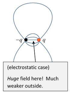
But recall that we found for the electric dipole that the very strong field between the two charges made a nonzero contribution to the integral of the electric field over space, even in the limit of going to a point dipole. This necessitated adding an extra term $\frac{1}{4\pi {\epsilon }_0}\left(-\frac{4\pi }{3}\overrightarrow{p}\delta \left(\overrightarrow{r}\right)\right)$ to the electric field.  (Details here.)

Is there a corresponding term for the magnetic dipole?  There certainly should be, because the argument about the intense local field between the two poles should apply here too$—$we’d expect to find the analogous term (?)

$$\frac{{\mu }_0}{4\pi }\left(-\frac{4\pi }{3}\overrightarrow{m}\delta \left(\overrightarrow{r}\right)\right)=-\frac{{\mu }_0}{3}\overrightarrow{m}\delta \left(\overrightarrow{r}\right).$$

But we know this can't be quite right$—$the N, S poles in the magnetic dipole are essentially the ends of a tiny solenoid, not separate entities. We know $\overrightarrow{\nabla }\cdot \overrightarrow{B}=0$.

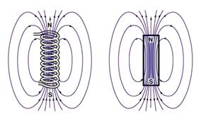
(This image from Wikimedia Commons, Geek3.)

Still, the magnetic field outside the (extremely small and thin) solenoid should look exactly like the electric dipole field, including the intense field between the poles$—$but now in addition we must include the field inside the solenoid.

That internal field will make a contribution  ${\displaystyle \underset{\text{inside solenoid}}{\int }\overrightarrow{B}\left(\overrightarrow{r}\right)d^{3}r}$ and it will be another delta function at the origin when we take the limit of a point dipole.  Let’s calculate this extra contribution.  Putting the solenoid directly across from N to S, we treat the ends of the solenoid as magnetic monopoles of strength $p_{\text{mag}},$ separated by $\overrightarrow{\delta },$ as far as the field outside the solenoid is concerned, so the dipole magnetic moment is

$\overrightarrow{m}=p_{\text{mag}}\overrightarrow{\delta }$

Working backwards from our expression for the dipole field, comparing the electric and magnetic dipole expressions, we see that the N pole of the solenoid must have a field flowing out

$$\overrightarrow{B}\left(\overrightarrow{r}\right)=\frac{{\mu }_0}{4\pi }\frac{p_{\text{mag}}\widehat{\overrightarrow{r}}}{r^2},$$

 from which the total outward flow of magnetic field from the N pole is ${\mu }_0{p}_{\text{mag}}.$ 

This, then, must be the total flux (magnetic field) going through the solenoid.  The inside field points in the direction of the dipole, the solenoid has length $\delta ,$ so the contribution to the delta function at the origin the ${\displaystyle \int \overrightarrow{B}\left(\overrightarrow{r}\right)}{d}^{3}r,$ is ${\mu }_0{p}_{\text{mag}}\overrightarrow{\delta }={\mu }_0\overrightarrow{m}.$ 

Hence the delta function at the origin for the magnetic dipole is

$-\frac{1}{3}{\mu }_0\overrightarrow{m}\delta \left(\overrightarrow{r}\right)+{\mu }_0\overrightarrow{m}\delta \left(\overrightarrow{r}\right)=\frac{2}{3}{\mu }_0\overrightarrow{m}\delta \left(\overrightarrow{r}\right).$

But does this matter?  We’re obsessing about the coefficient of a delta function at the origin, does it have any physical consequences?  The answer is yes$—$an important one!  For a hydrogen atom (not molecule) in the ground state, there is an interaction between the electron’s magnetic dipole moment and the proton’s. The electron has a spherically symmetric wave function, so averaged over the proton’s dipole field, away from the origin, $〈{\overrightarrow{m}}_e\cdot {\overrightarrow{B}}_p〉=0.$ But the electron has probability ${\left|{\psi }_e\left(0\right)\right|}^2$ of being at the origin, therefore the magnetic interaction energy of the two moments is

$E=-\frac{2{\mu }_0}{3}{\overrightarrow{m}}_e\cdot {\overrightarrow{m}}_p{\left|{\psi }_e\left(0\right)\right|}^2.$

So there is an energy difference between the proton and electron magnetic moments (both spin one-half particles, of course) being parallel and antiparallel. It turns out to be small: the photon emitted on falling from the excited state to the ground state has a wavelength of 21 cm.  This then is the signature of interstellar monatomic hydrogen: in fact, mapping the intensity of this radiation in the sky revealed for the first time the spiral structure of our galaxy. Unlike light, this microwave radiation (1420MHz) can penetrate dust clouds, etc.

Bottom line: the existence of the interstellar 21 cm line means the "small solenoid" (or some equivalent) term must be added to the electron dipole field delta function at the origin.

The Magnetostatic Maxwell Equations

Apart from the mysteries of particle magnetic moments, magnetic fields are generated by moving charges.  Magnetostatics is concerned with systems having only steady current flow (and therefore unchanging charge densities, although charge densities are infrequent in magnetostatic problems anyway).  We’ll use the symbol $\overrightarrow{j}$ for current density, in units coulombs per second per square meter cross-section, a.k.a. Ampères per square meter. 

Charge conservation gives $\partial \rho /\partial t+\overrightarrow{\nabla }\cdot \overrightarrow{j}=0$ and for magnetostatics

$\overrightarrow{\nabla }\cdot \overrightarrow{j}=0.$

The Maxwell equations for magnetostatics, a result of many experiments, are:

$\begin{array}{c}\overrightarrow{\nabla }\cdot \overrightarrow{B}\left(\overrightarrow{r}\right)=0,\\ \overrightarrow{\nabla }\times \overrightarrow{B}\left(\overrightarrow{r}\right)={\mu }_0\overrightarrow{j}\left(\overrightarrow{r}\right).\end{array}$

The first equation is the well-established non-existence of magnetic monopoles.

(We’ll see in a while, though, that it is sometimes useful (despite $\overrightarrow{\nabla }\cdot \overrightarrow{B}=0$ ) to represent magnetic material with changing degrees of magnetization in terms of “magnetic matter”, densities of “magnetic charge”.  This used to be called Poisson’s Imaginary Magnetic Matter, and is useful in understanding field configurations from magnetized materials.  It’s analogous to the net charge density in electrostatics from changing polarizations, except in the electric case there really is a charge density.  We’ll return to this later in the course.)

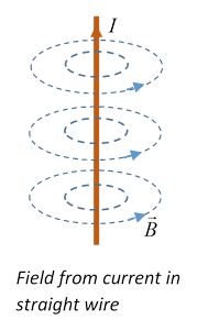
The second equation, $\overrightarrow{\nabla }\times \overrightarrow{B}\left(\overrightarrow{r}\right)={\mu }_0\overrightarrow{j}\left(\overrightarrow{r}\right),$ was established by Ampère, measuring the magnetic field from various arrangements of electric currents: for example, a current in a long straight wire gives a circling field of strength that goes down linearly with radial distance from the wire, and a field strength linear in the current strength.

 

Reminder: the direction of the field (see diagram) is given by the right-hand rule: if your right thumb is pointing in the direction of current flow, curling your fingers shows the direction of the generated field.  

 

Do Permanent Magnets Have Molecular Currents?

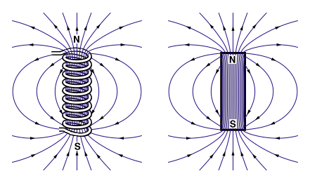
Current going around a loop circuit generates a magnetic field that tends to a dipole pattern at distances large compared with the size of the loop.(We'll review this shortly.) A stack of loops, meaning a solenoid, looks like a bar magnet, except that this time it’s hollow, so it’s easy to measure the field inside with some kind of probe.

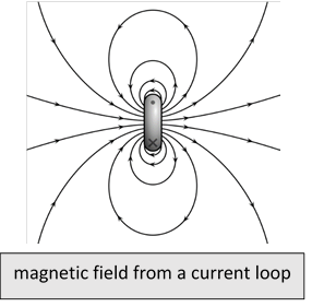
(This image from Wikimedia Commons, Geek3.)

This led Ampère to theorize that in fact regular bar magnets themselves are made up of “molecular current loops”.  It was clear that a bar magnet doesn’t have just an accumulation of N and S monopoles at the two ends, since if you break the bar in half, new poles appear at the new ends, just as you’d expect from Ampère’s molecular current loop model.  

Actually, we now understand the current loop picture isn’t quite correct: it’s true that an electron circling a nucleus is a small current loop, and consequently has a dipole field, but in solids the orbital motion is often balanced by other electrons circling in the opposite direction, or quenched by non-spherically symmetric crystal fields, Bragg reflecting the orbiting electrons into standing wave patterns.  In fact, most magnetic phenomena arise from the magnetic moments of the electrons themselves: they are, after all, charged objects with spin, but the naïve picture of how this would generate a dipole is wrong$—$it is necessary to go to relativistic quantum mechanics, specifically the Dirac equation, to understand the interaction of electron spin with an external magnetic field.  For now, you’ll have to take the electron’s magnetic dipole moment as a given.

The second Maxwell equation for magnetostatics in integral form is called Ampère’s law:

${\displaystyle \underset{C}{\oint }\overrightarrow{B}\cdot d\overrightarrow{l}}={\mu }_0{\displaystyle \underset{S}{\int }\overrightarrow{j}\cdot \widehat{\overrightarrow{n}}dS}$.

Magnetic Field from a Current Distribution: the Biot-Savart Law

From the two basic equations,

$\overrightarrow{\nabla }\cdot \overrightarrow{B}\left(\overrightarrow{r}\right)=0,\overrightarrow{\nabla }\times \overrightarrow{B}\left(\overrightarrow{r}\right)={\mu }_0\overrightarrow{j}\left(\overrightarrow{r}\right)$,

the Helmholtz theorem (discussed earlier) gives:

$$\begin{array}{c}\overrightarrow{B}\left(\overrightarrow{r}\right)={\overrightarrow{\nabla }}_{\overrightarrow{r}}\times \frac{1}{4\pi }{\displaystyle \int d^3{r}^{\prime }}\frac{{\overrightarrow{\nabla }}^{\prime }\times \overrightarrow{B}\left({\overrightarrow{r}}^{\prime }\right)}{\left|\overrightarrow{r}-{\overrightarrow{r}}^{\prime }\right|}+{\overrightarrow{\nabla }}_{\overrightarrow{r}}\cdot \frac{1}{4\pi }{\displaystyle \int d^3{r}^{\prime }}\frac{{\overrightarrow{\nabla }}^{\prime }\cdot \overrightarrow{B}\left({\overrightarrow{r}}^{\prime }\right)}{\left|\overrightarrow{r}-{\overrightarrow{r}}^{\prime }\right|}\\ ={\overrightarrow{\nabla }}_{\overrightarrow{r}}\times \frac{{\mu }_0}{4\pi }{\displaystyle \int d^3{r}^{\prime }}\frac{\overrightarrow{j}\left({\overrightarrow{r}}^{\prime }\right)}{\left|\overrightarrow{r}-{\overrightarrow{r}}^{\prime }\right|}.\end{array}$$

Now, that external curl operates on $\overrightarrow{r},$ not ${\overrightarrow{r}}^{\prime },$ so we can take it inside the integral (with a sign change since we switch the order of the vectors in the cross product ${\overrightarrow{\nabla }}_{\overrightarrow{r}},\overrightarrow{j}\left({\overrightarrow{r}}^{\prime }\right)$ ) to get

$\begin{array}{c}\overrightarrow{B}\left(\overrightarrow{r}\right)=-\frac{{\mu }_0}{4\pi }{\displaystyle \int d^3{r}^{\prime }}\overrightarrow{j}\left({\overrightarrow{r}}^{\prime }\right)\times {\overrightarrow{\nabla }}_{\overrightarrow{r}}\frac{1}{\left|\overrightarrow{r}-{\overrightarrow{r}}^{\prime }\right|}\\ =\frac{{\mu }_0}{4\pi }{\displaystyle \int d^3{r}^{\prime }}\frac{\overrightarrow{j}\left({\overrightarrow{r}}^{\prime }\right)\times \left(\overrightarrow{r}-{\overrightarrow{r}}^{\prime }\right)}{{\left|\overrightarrow{r}-{\overrightarrow{r}}^{\prime }\right|}^3}.\end{array}$

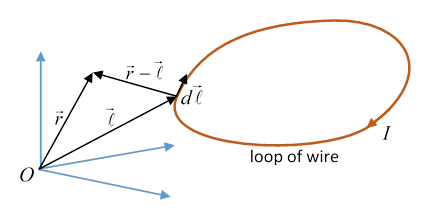
In particular, if the current is just $I$ amps along a thin wire,          

$\overrightarrow{B}\left(\overrightarrow{r}\right)=\frac{{\mu }_{0}I}{4\pi }{\displaystyle \int \frac{d\overrightarrow{l}\times \left(\overrightarrow{r}-\overrightarrow{l}\right)}{{\left|\overrightarrow{r}-\overrightarrow{l}\right|}^3}}$

where $\overrightarrow{l}$ is a vector pointing to a position on the wire.  This is the famous law of Biot and Savart.

The law does give the impression that, just as the electric field is a sum of parts from each increment of charge, which increment would produce its contribution to the electric field if all by itself, the magnetic field is similarly a sum of magnetic fields from each element of current.  But this is a deceptive parallel$—$the increments of current couldn’t exist alone, in contrast to the increments of charge.

Bearing this caveat in mind, it is useful to visualize the contribution to the magnetic field from the current element: it is perpendicular both to the vector direction $\overrightarrow{r}-\overrightarrow{l}$ to the current element, and to the current element itself (it’s a little vector, $Id\overrightarrow{l}$ ), and so circles in an azimuthal direction around the line direction of the current element.   It is strongest in the equatorial direction (meaning the direction perpendicular to the current element); going to zero in the direction parallel to the current element.

Force on a Current Element from a Magnetic Field

As we’ve discussed, Ampère did a series of experiments on magnetic fields and currents, in particular finding the forces and torques between two separate wire circuits, such as two long parallel wires carrying different currents.

We’ve given an expression for the magnetic field from an increment of current, now we need the force on an increment of current in a magnetic field$—$then we can compute the force between two currents.

To get some insight into what the force on a current element might be, imagine for a moment that you’ve found a monopole, strength $m,$ so in a field it experienced a force $m\overrightarrow{B},$ and produces its own field (exactly analogous to electric charge) ${\overrightarrow{B}}_{\text{monopole}}={\mu }_{0}m\overrightarrow{r}/4\pi r^3.$ The force on the monopole from the current element’s contribution to the field is

$m{\overrightarrow{B}}_{\text{current}}=\left({\mu }_{0}mI/4\pi \right)d\overrightarrow{l}\times \overrightarrow{r}/r^3,$

 and the force on the current element from the monopole has to be equal and opposite, from which

$d\overrightarrow{F}=I\left(d\overrightarrow{l}\times \overrightarrow{B}\right).$

That is, the force is perpendicular both to the current element and to the local magnetic field direction.  Of course, this is just the same as the Lorentz force $q\overrightarrow{v}\times \overrightarrow{B}$ on a single charge mentioned earlier.  (You don’t of course need to have a monopole$—$that was just to keep the field, and therefore the argument, as simple as possible.)

Force Between Current Circuits

We’re now ready to write down the force between two current circuits:

$${\overrightarrow{F}}_{12}=\frac{{\mu }_0{I}_1{I}_2}{4\pi }{\displaystyle \int \frac{d{\overrightarrow{l}}_1\times \left(d{\overrightarrow{l}}_2\times {\overrightarrow{r}}_{12}\right)}{{\left|{\overrightarrow{r}}_{12}\right|}^3}}.$$

This can be written in a manifestly symmetrical fashion using

$$\frac{d{\overrightarrow{l}}_1\times \left(d{\overrightarrow{l}}_2\times {\overrightarrow{r}}_{12}\right)}{{\left|{\overrightarrow{r}}_{12}\right|}^3}=-\left(d{\overrightarrow{l}}_1\cdot d{\overrightarrow{l}}_2\right)\frac{{\overrightarrow{r}}_{12}}{{\left|r_{12}\right|}^3}+d{\overrightarrow{l}}_2\left(\frac{d{\overrightarrow{l}}_1\cdot {\overrightarrow{r}}_{12}}{{\left|r_{12}\right|}^3}\right)$$ .

Putting this in the integral, notice the second term includes the integral

${\displaystyle \oint \frac{d{\overrightarrow{l}}_1\cdot {\overrightarrow{r}}_{12}}{{\left|r_{12}\right|}^3}\equiv {\displaystyle \oint d\overrightarrow{l}}}\cdot \overrightarrow{\nabla }\left(\frac{1}{r}\right)=0,$

which must give a zero contribution since it is a gradient around a complete circuit, and the singular behavior at $r=0$ is avoided, since the wires cannot come into physical contact with each other.

So, only the first term remains, and it is manifestly symmetric:

$${\overrightarrow{F}}_{12}=-\frac{{\mu }_0{I}_1{I}_2}{4\pi }{\displaystyle \int \left(d{\overrightarrow{l}}_1\cdot d{\overrightarrow{l}}_2\right)\frac{{\overrightarrow{r}}_{12}}{{\left|r_{12}\right|}^3}}.$$

Force Between Parallel Currents: Defining the Unit of Current (the Old-Fashioned Way)

Old Fashioned because from 2019, this previously standard definition has been abandoned. From now on, the coulomb is defined by stating that the electron’s charge is 1.602176634 x 10^-19 coulombs. Of course, this changes ${\mu }_0/4\pi$ by of order one part in a billion from its previously defined value of 10^-7.

It’s easy to do the integral for two long parallel wires distance $d$ apart to find force per unit length of wire is

$f_{12}=\left({\mu }_0/2\pi \right)I_1{I}_2/d.$

(Integral hint: Take a point on the second wire, integrate over the first wire using the variable $\theta$ in the diagram.)

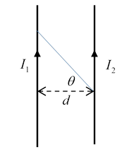
In fact, taking ${\mu }_0/4\pi ={10}^{-7}$,  this force, first measured experimentally by Ampère himself, defined the unit of current, now the ampère, and hence the unit of charge, the coulomb.  One ampère is a current flow of one coulomb per second (still).

This is also in contrast to the older (Gaussian) electrostatic system, where the unit of charge was defined as the charge that repelled a similar charge with a force of one dyne at a distance of one centimeter. Definitely not true of the coulomb!  Not to mention that particle (and maybe atomic) guys take the electron charge to be unity…

From the force on a current element in a magnetic field $d\overrightarrow{F}=I\left(d\overrightarrow{l}\times \overrightarrow{B}\right),$ since any general current distribution in space can be expressed as a sum over such elements, the force and torque on a steady current density $\overrightarrow{j}\left(\overrightarrow{r}\right)$ in a field $\overrightarrow{B}\left(\overrightarrow{r}\right)$ are clearly

$\overrightarrow{F}={\displaystyle \int \overrightarrow{j}\left(\overrightarrow{r}\right)\times \overrightarrow{B}\left(\overrightarrow{r}\right)}{d}^{3}r,\overrightarrow{N}={\displaystyle \int \overrightarrow{r}\times \left(\overrightarrow{j}\left(\overrightarrow{r}\right)\times \overrightarrow{B}\left(\overrightarrow{r}\right)\right)}{d}^{3}r.$ 

previous  index  next