previous  index  next 

37  Quasi-Static Magnetic Fields in Conductors

    Michael Fowler, UVa

The Approximation We’re Making…

We’re finally moving from electrostatics and magnetostatics towards the full dynamic Maxwell equations$—$but gently.  In this section, we include the non-conservative electric field generated by a changing magnetic field, but we do not include the magnetic field from a changing electric field.  Since Maxwell’s equations seem to put the two on a more or less equal footing, that seems an arbitrary choice, but in fact it makes sense: in conductors on the length and time scale of electric motors and generators, the electric field from wires moving relative to magnets plays the central role. On the other hand, the magnetic field from the changing electric fields is negligible compared to the magnetic fields already present.

In the conductors of interest, the currents obey Ohm’s law, so the equations are:

$$\overrightarrow{\nabla }\times \overrightarrow{H}=\overrightarrow{j},\overrightarrow{\nabla }\cdot \overrightarrow{B}=0,\overrightarrow{\nabla }\times \overrightarrow{E}=-\partial \overrightarrow{B}/\partial t,\overrightarrow{j}=\sigma \overrightarrow{E}.$$  Writing

$$\overrightarrow{\nabla }\times \overrightarrow{E}=-\partial \overrightarrow{B}/\partial t=-\overrightarrow{\nabla }\times \left(\partial \overrightarrow{A}/\partial t\right),$$  we have

$$\overrightarrow{\nabla }\times \left(\overrightarrow{E}+\partial \overrightarrow{A}/\partial t\right)=0,$$  so we can write

$$\overrightarrow{E}=-\partial \overrightarrow{A}/\partial t-\overrightarrow{\nabla }\phi .$$ In the present quasi-magnetostatic context, there is negligible electrostatically unbalanced charge in conductors, the electric field is essentially all from the changing magnetic field, so we can drop the $\overrightarrow{\nabla }\phi .$  

..Leads to a Diffusion Equation

If we can assume uniform permeability $\mu ,$ then

$$\overrightarrow{\nabla }\times \overrightarrow{B}=\mu \overrightarrow{j}=\mu \sigma \overrightarrow{E}.$$  With no net charge density present, we are automatically in the Coulomb gauge, since from $\overrightarrow{E}=-\partial \overrightarrow{A}/\partial t,$ $\overrightarrow{\nabla }\cdot \overrightarrow{E}=0$ means $\overrightarrow{\nabla }\cdot \overrightarrow{A}=0.$ (There could be an arbitrary constant term$—$that can be safely dropped.)

Therefore,

$${\nabla }^2\overrightarrow{A}=\mu \sigma \frac{\partial \overrightarrow{A}}{\partial t}.$$  We will assume the conductivity can be taken to be frequency-independent in the relevant frequency range.

This is a diffusion equation$—$that is, it’s the same equation as that describing heat flow in an unevenly warmed heat conducting material.  But there is one tricky point in making an analogy with heat diffusion.  For heat energy, the better the heat conductivity, the quicker the diffusion. That’s also the case for diffusion of electric charge in a conductor$—$but it’s not the case for diffusion of a magnetic field in a conductor! The point is that as the field decays, from Lenz’ law it induces currents opposing and thus slowing the decay. The better the conductivity, the more powerful and effective these opposing currents are, and the slower the decay.

An order-of-magnitude estimate of the times involved follows from dimensional analysis of the equation.

For a system of size $L,$ glancing at the diffusion equation, we see that dimensionally the time of decay will be of order $\tau \sim \mu \sigma L^2.$ Jackson gives two examples: for a small (1 cm) copper sphere $\left(\mu \sim {10}^{-6},\sigma \sim {10}^8\right),$ the time comes out of order milliseconds.  If we now consider the Earth’s magnetic field as generated in the Earth’s central iron core, radius 1000 km, and take the conductivity the same as copper, we find a time of order a hundred thousand years. This is in fact the timescale on which the field reverses, but this is complicated magnetohydrodynamics, so it’s hard to know how seriously to take the result.  Not to mention that the Sun’s field reverses every eleven years…perhaps this is all a bit more complicated…

Skin Depth and Eddy Currents

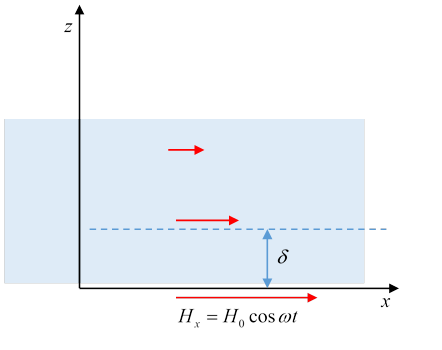
(This diagram follows Jackson’s text description. His own diagram seems to be upside-down.)

A semi-infinite conductor, $\mu ,\sigma ,$ fills the space $z>0,$ and is subject to magnetic field at its boundary $z=0.$ The field is in the $x$ -direction, $H_x\left(t\right)=H_0\cos \omega t.$ So it will be the same field just inside, at $z=0+.$

It’s convenient to use complex notation,

$$H_x\left(z,t\right)=h\left(z\right)e^{-i\omega t}$$  which satisfies

$$\left(\frac{d^2}{d{z}^2}+i\mu \sigma \omega \right)h\left(z\right)=0.$$  A solution $e^{ikz}$ works provided $k^2=i\mu \sigma \omega ,$ or $k=\pm \left(1+i\right)\sqrt{\frac{\mu \sigma \omega }{2}}.$ 

The solution has to be the sign giving exponential decay of the field into the conductor, that gives a decay length

$$\delta =\sqrt{\frac{2}{\mu \sigma \omega }}.$$  This is called the “skin depth”. Quoting Jackson, for copper $\left(\sigma \sim 6\times {10}^7\text{ S/m}\right)$ it’s $0.065/\sqrt{\nu \text{(Hz)}}\text{ m,}$ meaning 8 mm at the usual AC frequency, and microns at microwave frequencies. On the other hand, for seawater $\left(\sigma \sim 5\text{ S/m}\right)$ it’s $240/\sqrt{\nu \text{(Hz)}}\text{ m,}$ of order 1 cm at microwave frequencies (2.45GHz), and possibly a rough guide for food in a microwave oven.

In terms of $\delta ,$ the field in the conductor is

$$H_x\left(z,t\right)=H_0{e}^{-z/\delta }\cos \left(z/\delta -\omega t\right).$$  From $\overrightarrow{\nabla }\times \overrightarrow{H}=\overrightarrow{j}=\sigma \overrightarrow{E},$ there is an accompanying electric field:

$$E_y=\frac{1}{\sigma }\frac{d{H}_x}{dz}=\frac{-1+i}{\sigma \delta }{H}_0{e}^{-z/\delta }{e}^{iz/\delta -i\omega t}$$  and putting $1/\sigma \delta =\mu \delta \omega /2,$ 

$$E_y=\frac{\mu \omega \delta }{\sqrt{2}}{H}_0{e}^{-z/\delta }\cos \left(z/\delta -\omega t+3\pi /4\right).$$  This is inductive heating (as in a microwave): $P_{\text{resistive}}=〈\overrightarrow{j}\cdot \overrightarrow{E}〉=\frac{1}{2}\mu \omega H_0^2{e}^{-2z/\delta }.$  

Diffusion of Magnetic Fields in Conducting Media

(Jackson p 221). He takes two parallel sheets of (opposite) current distance $a$ apart, so there is a uniform magnetic field between them and none outside, then switches them off, so the field diffuses outward. Therefore, what we really have is a simple one-dimensional diffusion equation, the only parameters are $\mu ,\sigma$ and the given scale length $a,$ from the diffusion equation the decay rate is $\nu ={\left(\mu \sigma a^2\right)}^{-1},$ the result is $H_x\left(z,t\right)=\frac{H_0}{\sqrt{\pi \nu t}}{e}^{-z^2/4\nu t{a}^2}$ plus corrections since we started with a slab of field of finite thickness. This is just the ordinary diffusion equation:  the sum of many random walks starting at the origin at the same time, how they’re spread out at a later time. To account for the initial finite thickness, we could convolute the point-source diffusion function with that initial spatial configuration.

previous  index  next