previous  index  next 

36  Magnetic Field Energy and Inductance

    Michael Fowler, UVa

Jackson 5.16, 17

Energy in the Magnetic Field

If we connect a solenoid (a simple coil of wire) to the two terminals of a battery,

 a current begins to flow, a magnetic field resembling that of a bar magnet starts building up, and this changing magnetic field generates an electric field opposing the increasing current$—$this is Lenz’ law. It means the battery has to expend energy against this electric field to build up the magnetic field. But energy is conserved$—$so where did that energy go?

The answer becomes evident on disconnecting the coil from the battery: there will be a spark!  A typical battery, a few volts, cannot produce a spark like the one you see: the decaying magnetic field is generating a much greater voltage attempting to keep the current going, the so-called “back emf”: Lenz’ law again.  This spark dissipates a lot of energy$—$and that energy was evidently stored in the magnetic field.

Calculating the Field Energy from Faraday's Law

To find the energy stored in a magnetic field, we need to build it up from scratch, turning on currents gradually (we are not considering permanent magnets here, just fields from free currents).  As we increase the current, from Faraday’s law the changing magnetic field generates an opposing emf$—$forcing the battery to do work$—$and this is the work stored as field energy.  (Of course, we’ll also be doing work maintaining the current against ohmic resistance, but that goes to heat, and is usually small in this context, so we’re neglecting it here.)  The rate of working required to maintain a current $I$ against an emf $E$ is $IE$, that’s the number of charges per second climbing through that potential.  

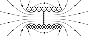
Imagining now a general steady current distribution in space, confined to the gray area in the diagram. 

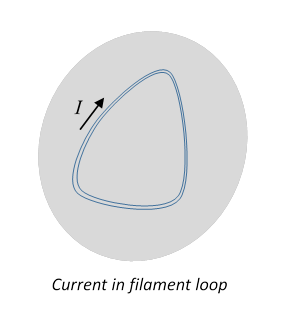
We will assume that this swirling but time-invariant pattern of currents can be represented as a set of closed currents going around filament loops, these filaments being like narrow tubes, in general of varying cross section.  

The magnetic field from the current distribution is linear in the currents: if we double all the currents, we double the field everywhere.

Suppose now we have a current density in the volume $\overrightarrow{j}\left(\overrightarrow{r}\right)$ and we scale it up incrementally in time $\delta t$ say,

$\overrightarrow{j}\left(\overrightarrow{r}\right)\to \left(1+\epsilon \right)\overrightarrow{j}\left(\overrightarrow{r}\right)=\overrightarrow{j}\left(\overrightarrow{r}\right)+\delta \overrightarrow{j}\left(\overrightarrow{r}\right).$ 

The magnetic field will change correspondingly,

$\overrightarrow{B}\left(\overrightarrow{r}\right)\to \left(1+\epsilon \right)\overrightarrow{B}\left(\overrightarrow{r}\right)=\overrightarrow{B}\left(\overrightarrow{r}\right)+\delta \overrightarrow{B}\left(\overrightarrow{r}\right).$ 

This changing field threading the current loops generates emfs $E$ opposing the currents, and to maintain the currents will take energy terms $EI$ supplied by the battery.

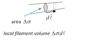
Take one loop having variable cross-section area $\Delta \sigma ,$ and local current density $\overrightarrow{j},$ but the total loop current

$$I=j\Delta \sigma$$

is of course the same all the way around. 

From Faraday’s law, the momentary induced emf in this loop is

$$E_{\text{loop}}=-\frac{d}{dt}{\displaystyle \int \overrightarrow{B}\cdot \widehat{\overrightarrow{n}}da}=-{\displaystyle \int \frac{\delta \overrightarrow{B}}{\delta t}\cdot \widehat{\overrightarrow{n}}da}$$  where the integral is over a surface spanning the loop.

Therefore, the energy fed to the loop current by the battery in time $\delta t$ is

$\begin{array}{c}\delta W=-I{E}_{\text{loop}}\delta t=j\Delta \sigma {\displaystyle \underset{S}{\int }\widehat{\overrightarrow{n}}\cdot \delta \overrightarrow{B}da}\\ =j\Delta \sigma {\displaystyle \underset{S}{\int }\widehat{\overrightarrow{n}}\cdot \overrightarrow{\nabla }\times \delta \overrightarrow{A}da=}{\displaystyle \underset{C}{\oint }j\Delta \sigma \delta \overrightarrow{A}\cdot d\overrightarrow{\ell }},\end{array}$ 

where we’ve written the field in terms of the vector potential,  $\overrightarrow{B}=\overrightarrow{\nabla }\times \overrightarrow{A}.$ 

Now writing

$$j\Delta \sigma d\overrightarrow{\ell }=\overrightarrow{j}{d}^{3}x$$

 and integrating over the space containing all the currents, the total work done maintaining them against the magnetic potential change $\delta \overrightarrow{A}$ is

$\delta W={\displaystyle \int \delta \overrightarrow{A}\cdot \overrightarrow{j}{d}^{3}x=\frac{1}{{\mu }_0}}{\displaystyle \int \delta \overrightarrow{A}\cdot \left(\overrightarrow{\nabla }\times \overrightarrow{B}\right)d^{3}x=\frac{1}{{\mu }_0}}{\displaystyle \int \left[\overrightarrow{B}\cdot \left(\overrightarrow{\nabla }\times \delta \overrightarrow{A}\right)+\overrightarrow{\nabla }\cdot \left(\overrightarrow{B}\times \delta \overrightarrow{A}\right)\right]}{d}^{3}x$

Exercise:  Check the vector identity used.

For a localized field the second integral is zero (it’s equal to a surface integral at infinity), leaving

$$\delta W=\frac{1}{{\mu }_0}{\displaystyle \int \overrightarrow{B}\cdot \delta \overrightarrow{B}{d}^{3}x},$$  so

$$W=\frac{1}{2{\mu }_0}{\displaystyle \int {\overrightarrow{B}}^2{d}^{3}x},$$  analogous to the expression we found for the energy in an electrostatic field.

Magnetic Field Energy as a Function of the Currents

If we simply integrate $\delta W={\displaystyle \int \delta \overrightarrow{A}\cdot \overrightarrow{j}{d}^{3}x},$ we find

$$W=\frac{1}{2}{\displaystyle \int \overrightarrow{A}\cdot \overrightarrow{j}{d}^{3}x}.$$

(This is the vector analog of the electrostatic equation $U=\frac{1}{2}{\displaystyle \int \phi \left(\overrightarrow{r}\right)}\rho \left(\overrightarrow{r}\right)d^{3}x.$ )

A much more practical expression from an engineering point of view is to express the energy entirely in terms of the currents (easily controlled and measurable), using

$$\overrightarrow{A}\left(\overrightarrow{r}\right)=\frac{{\mu }_0}{4\pi }{\displaystyle \int d^3{r}^{\prime }}\frac{\overrightarrow{j}\left({\overrightarrow{r}}^{\prime }\right)}{\left|\overrightarrow{r}-{\overrightarrow{r}}^{\prime }\right|},$$

to find

$$W=\frac{1}{2}{\displaystyle \int \overrightarrow{j}\left(\overrightarrow{r}\right)\cdot \overrightarrow{A}\left(\overrightarrow{r}\right)}{d}^{3}r=\frac{{\mu }_0}{8\pi }{\displaystyle \int d^{3}r{\displaystyle \int d^3{r}^{\prime }}\frac{\overrightarrow{j}\left(\overrightarrow{r}\right)\cdot \overrightarrow{j}\left({\overrightarrow{r}}^{\prime }\right)}{\left|\overrightarrow{r}-{\overrightarrow{r}}^{\prime }\right|}}.$$

Inductances of Wire Circuits

Suppose now we have a system of $N$ wire circuits (meaning thin conducting wires), the $i^{\text{th}}$ one carrying current $I_i.$  

The total magnetic energy $W$ of the system is clearly quadratic in the currents: we define the self and mutual inductances $L_i,M_{ij}$ by writing

$$W=\frac{1}{2}{\displaystyle \sum _{i=1}^N{L}_i{I}_i^2+{\displaystyle \sum _{i,j>i}^N{M}_{ij}{I}_i{I}_j}},$$  so the self-inductance

$$L_i=\frac{{\mu }_0}{4\pi I_i^2}{\displaystyle \int d^3{r}_i{\displaystyle \int d^3{r^{\prime }}_i}\frac{\overrightarrow{j}\left({\overrightarrow{r}}_i\right)\cdot \overrightarrow{j}\left({{\overrightarrow{r}}^{\prime }}_i\right)}{\left|{\overrightarrow{r}}_i-{{\overrightarrow{r}}^{\prime }}_i\right|}},$$  and the mutual inductance

$$M_{ij}=\frac{{\mu }_0}{4\pi I_i{I}_j}{\displaystyle \int d^3{r}_i{\displaystyle \int d^3{r^{\prime }}_j}\frac{\overrightarrow{j}\left({\overrightarrow{r}}_i\right)\cdot \overrightarrow{j}\left({{\overrightarrow{r}}^{\prime }}_j\right)}{\left|{\overrightarrow{r}}_i-{{\overrightarrow{r}}^{\prime }}_j\right|}}.$$  These volume integrals are of course restricted to the volume of the actual conductor in each circuit, so for reasonably thin wires (compared with the scale of the circuits), using

$${\overrightarrow{A}}_j\left({\overrightarrow{r}}_i\right)=\frac{{\mu }_0}{4\pi }{\displaystyle \int d^3{r^{\prime }}_j}\frac{{\overrightarrow{j}}_j\left({{\overrightarrow{r}}^{\prime }}_j\right)}{\left|{\overrightarrow{r}}_i-{{\overrightarrow{r}}^{\prime }}_j\right|},$$

 we can write

$$M_{ij}=\frac{1}{I_i{I}_j}\cdot I_i{\displaystyle \underset{C_i}{\oint }{\overrightarrow{A}}_j\cdot d\overrightarrow{\ell }}=\frac{1}{I_j}{\displaystyle \underset{S_i}{\int }\left(\overrightarrow{\nabla }\times {\overrightarrow{A}}_j\right)\cdot \widehat{\overrightarrow{n}}da},$$ 

using Stokes' theorem in the last step.

That is, the mutual inductance of circuits $i$ and $j$ is the total magnetic flux through circuit $i$ from a unit current flowing around circuit $j.$   This doesn’t sound very symmetrical, but it must be, because we began from a completely symmetrical expression.

Exercises: 1. Take as circuits two concentric circles of thin wire in a plane, one circle having radius ten times the other. Draw two magnetic field diagrams: one with unit current in the larger circle, the other unit current in the smaller one. Convince yourself qualitatively that the mutual inductance is symmetrical.

2.  Notice that in the expression for the total energy $W=\frac{1}{2}{\displaystyle \sum _{i=1}^N{L}_i{I}_i^2+{\displaystyle \sum _{i,j>i}^N{M}_{ij}{I}_i{I}_j}},$ if the currents have opposite signs the contribution from mutual inductance is negative. The total energy must be positive for nonzero currents, so for given $L_1,L_2$ there must be a maximum allowed value of $M_{12}.$ What is it?

Finally, notice that in the thin wire limit, we can write

$$M_{ij}=\frac{{\mu }_0}{4\pi }{\displaystyle \int \overrightarrow{d\ell }{\displaystyle \int \overrightarrow{d{\ell }^{\prime }}}\frac{\overrightarrow{d\ell }\cdot \overrightarrow{d{\ell }^{\prime }}}{\left|\overrightarrow{r}-{\overrightarrow{r}}^{\prime }\right|}},$$

making clear that in this limit it’s just a geometrical construct.

Estimating Self Inductance of a Circuit

Following Jackson, estimating the mutual inductance of two circuits is fairly straightforward provided the wires’ thicknesses are small compared with the scale of the system.  Self-inductance is more problematic, because of the strong variations in field strength close to the wire. The safest approach is in terms of the total field energy:

$$\frac{1}{2}L{I}^2=\frac{1}{2{\mu }_0}{\displaystyle \int {\overrightarrow{B}}^2{d}^{3}r.}$$  (Of course, a significant part of the magnetic field energy is inside the wire, so is it OK to use the vacuum value ${\mu }_0$?  It turns out to be fine for the usual wire materials, copper and aluminum. Adjustments will need to be made for the unusual case of currents in iron or nickel wires.  We’ll discuss this in much more detail next semester.)

To find the total stored energy in the magnetic field, we need to evaluate it in three separate regions:

1.  Inside the wire,

2.  Close to the wire (from the surface to some distance ${\rho }_{\text{max}}$ where non-straightness of the wire must be adjusted for, typically of order the size of the circuit)

3.  Further away.

The magnetic field near (and inside) the wire is

$$B_{\varphi }=\frac{{\mu }_{0}I}{2\pi a}\cdot \frac{{\rho }_{<}}{{\rho }_{>}}$$  Here ${\rho }_{<}\left({\rho }_{>}\right)$ is the lesser (greater) of wire radius $a$ and distance from the central line $\rho .$ 

The contributions to the inductance per unit length of wire from stored field energy inside the wire and outside are:

$$L_{\text{in}}=\frac{{\mu }_0}{8\pi },L_{\text{out}}=\frac{{\mu }_0}{4\pi }\ln \left(\frac{{\rho }_{\text{max}}^2}{a^2}\right)$$  where ${\rho }_{\text{max}}^2\sim A,$ the area spanned by the circuit.  Fortunately, the integral is logarithmic, so not very sensitive to where we take the upper length cutoff.

Beyond the circuit size, the field tends to dipole form, contributing of order (per unit length of wire, we write $C,$ meaning circumference, for the total length)

$$\frac{4\pi }{{\mu }_{0}C}{\displaystyle \underset{{\rho }_{\text{max}}}{\overset{\infty }{\int }}{r}^2{\left(\frac{{\mu }_0}{4\pi }\cdot \frac{A}{r^3}\right)}^{2}dr}\approx \frac{{\mu }_0{A}^2}{4\pi {\rho }_{\text{max}}^{3}C}$$  and if we set ${\rho }_{\text{max}}=\sqrt{{\xi }^{\prime }A}$ with $\xi$ of order unity, then

$$L_{\text{dipole}}=O\left({\mu }_0\sqrt{A}/4\pi C\right).$$ 

previous  index  next