*40 “Derivation” of the Equations of Macroscopic Electromagnetism

Reviewing Jackson section 6.6

Introduction: Early Models and Quantum Limitations

We know that macroscopically, meaning on a human scale (say, lengths from a micron on up), the Maxwell equations for electric and magnetic fields in materials work well. They are (including the polarization and magnetization terms previously discussed):

$\begin{array}{l} \vec{\nabla} \cdot \vec{B} = 0, \vec{B} = μ \vec{H} = μ_{0} (\vec{H} + \vec{M}), \vec{\nabla} \times \vec{E} + \frac{\partial \vec{B}}{\partial t} = 0, \\ \vec{\nabla} \cdot \vec{E} = ρ / ε_{0}, \vec{\nabla} \cdot \vec{D} = ρ_{f}, \vec{D} = ε \vec{E} = ε_{0} \vec{E} + \vec{P}, \\ \vec{\nabla} \times \vec{B} = μ_{0} \vec{j} + \frac{1}{c^{2}} \frac{\partial \vec{E}}{\partial t}, \vec{\nabla} \times \vec{H} = {\vec{j}}_{f} + \frac{\partial \vec{D}}{\partial t} . \end{array}$

Here the subscript $f$ refers to free charges and currents, those not bound in molecules.

At the microscopic (atomic) level, every charge is individually accounted for (except that the nucleus is taken to be a point charge) so the polarization and magnetization terms are not there (they represented averages over displacement or orientation of many charges). We know that at this atomic level the equations are accurate: together with quantum mechanics, they accurately describe, for example, the spectrum of the hydrogen atom. And, the Maxwell equations also work very well in vacuum: using data from electrostatic and magnetostatic experimental results they accurately predict the speed of light, as Maxwell himself discovered.

Jackson writes these microscopic equations for the fields now labeled $\vec{b}, \vec{e}$ :

$\begin{array}{l} \vec{\nabla} \cdot \vec{b} = 0, \vec{\nabla} \times \vec{e} + \frac{\partial \vec{b}}{\partial t} = 0, \\ \vec{\nabla} \cdot \vec{e} = η / ε_{0}, \vec{\nabla} \times \vec{b} = \frac{1}{c^{2}} \frac{\partial \vec{e}}{\partial t} + μ_{0} \vec{j} . \end{array}$

Here $η, \vec{j}$ represent all charges and currents, so include those bound charges which give rise to polarization and magnetization.

We can see immediately that the first two equations imply their macroscopic equivalents: they don’t involve the charges. If microscopically there are no monopoles, you won’t find any at the macroscope scale either. But that’s not the whole story, even for these equations: the macroscopic fields $\vec{E}, \vec{B}$ we measure with our macroscopic equipment vary smoothly over volumes containing millions of atoms, whereas we know from atomic physics that $\vec{e}, \vec{b}$ vary wildly inside individual atoms and molecules. Therefore, to get from the microscopic equations to the macroscopic we need to do some averaging. We know the macroscopic Maxwell equations work well in analyzing refraction of light, but not of X-rays: the X-rays detect the microscopic structure, light doesn’t. So we should be averaging $\vec{e}$ over volumes containing of order at least a million atoms to get $\vec{E} .$ The simplest approach is to find the average over a spherical region, but have the edges fuzzed over say a distance of a few atoms to avoid sudden changes on slightly moving the center of the sphere. It is straightforward to check that this averaging commutes with differentiation, so, on averaging the first two microscopic equations, we get the corresponding macroscopic ones.

The second two equations, with this averaging (denoted by <>), become

$\begin{array}{l} ε_{0} \vec{\nabla} \cdot \vec{E} = 〈η (\vec{r}, t)〉, \\ \frac{1}{μ_{0}} \vec{\nabla} \times \vec{B} = ε_{0} \frac{\partial \vec{E}}{\partial t} + 〈\vec{j} (\vec{r}, t)〉 . \end{array}$

To make further progress towards the macroscopic equations at the beginning of this lecture, we need to separate the microscopic charges and currents into two categories: free ones, which correspond to the macroscopic free charges and currents, and bound ones, confined to individual molecules, these manifest themselves macroscopically in the polarization and magnetization of molecules.

The first real attempt to understand macroscopic electrodynamics of solids in terms of a molecular model was that of Lorentz, before quantum mechanics. He modeled the atom as an electron bound to a much more massive core by a linear spring, that is, a simple harmonic oscillator. This accounted for the (static) linear dielectric response to an electric field, the molecule (as he called it) becoming a dipole. He also shared the 1902 Nobel prize with his student Zeeman for explaining the Zeeman effect: the splitting of spectral lines (meaning oscillator frequencies) into three when a magnetic field is applied. In their simple oscillator model, the electron went in a circular orbit perpendicular to the magnetic field, or oscillated on a straight line parallel to the field (in which case the field did not affect the motion). (It should be added that a relatively short time later, examples were found of splitting into other than three lines $—$ the anomalous Zeeman effect $—$ and quantum mechanics was necessary to explain those new results.)

Lorentz went on to discuss his model’s interaction with electromagnetic waves, and realized that his “molecule” as he named the basic unit in constructing a solid, had to include oscillators of different frequencies to explain the observed dispersion. Significant further developments only came with quantum mechanics.

At almost exactly the same time, Drude explained the long-established Ohm’s law of conduction with a pinball-type model of free electrons, driven by the applied electric field, the electrons bouncing off atoms as they made their way down the wire. The basic result $(j = σ E)$ is of course correct (it had long been known) but a little later quantum mechanics completely changed the picture: the electrons in a good conductor are actually in very extended wavefunction states, their mean free path is typically hundreds of atomic distances, and they are only deflected by imperfections or vibrations in the lattice. Scattering is heavily restricted by the quantum exclusion principle $—$ states available for scattering into are very restricted.

A major advance in understanding the behavior of electrons in metals came with the discovery of electron spin: together with angular momentum quantization, it explained the anomalous Zeeman effect. Furthermore, electron spin, together with elementary quantum band theory, usually made clear which atomic lattices would be conductors, which insulators, and even which semiconductors.

Jackson’s Approach in 6.6: Classically Extend Those Early Models

Going back to Lorentz’s model, it’s clearly on the right track, we can understand how macroscopic polarization arises, but it’s only a first step. We know the molecules making up a solid are more complicated than a simple harmonic oscillator, just from their response to light, which is an oscillating driving force in this context.

Jackson, here following Russakoff, begins with Lorentz’s regular array of molecules but imagines the molecule as a collection of charged particles held together by some kind of bonds. This he envisions as a classical dynamical system. The molecule has a complex charge distribution, which can be resolved into multipoles: dipole, quadrupole, etc., in the usual way, and then, in the larger context of the solid as a whole, represented by point multipoles located at a central point in the molecule. When the average over all molecules is taken, this gives a charge density, a polarization (dipole) density, a quadrupole density, and so on.

This gives (his 6.92)

$D_{α} = ε_{0} E_{α} + P_{α} - \sum_{β} \frac{\partial {Q^{'}}_{α β}}{\partial x_{β}} + \dots$

Recalling how we found earlier that a variable polarization gave rise to a net charge density, we can see that a varying quadrupole moment will give rise to a dipole density, i.e. polarization, that’s the third term. However, rather anticlimactically, Jackson states (p 255) the third and higher terms are almost invariably negligible. So this isn’t getting us much beyond Lorentz.

Next, we need to extract current and magnetization from the molecular model. We must necessarily specify the positions and velocities of the charges $j n$ in each molecule $n,$ to get, for instance the molecular magnetic moment ${\vec{m}}_{n} = \sum_{j (n)} \frac{1}{2} q_{j} ({\vec{x}}_{j n} \times {\vec{v}}_{j n}) .$ Jackson does not go through the difficult details of the calculation, which he terms “gory” (page 255), and leaves to the devoted reader.

But I think there is a more fundamental problem. These molecules are classical objects. Why put in all this calculational effort on a deeply flawed model? It can’t possibly give a realistic representation of magnetism, which either comes from electron spin or quantized orbital motion, both quantum phenomena. This approach might possibly have appeared reasonable in the 1970’s, but surely not now. Quantum mechanics can’t be ignored in building a model of magnetism in solids. Even if somehow you derive reasonable looking equations, that’s just a mathematical exercise, with little relation to physics. To make real progress on this kind of problem you need to use more modern techniques, such as density functional theory. (OK, Jackson’s book is called Classical Electrodynamics, but still.)

A Moving Polarized Dielectric is Magnetic

We will, though, mention one equation near the end of section 6.6 that’s worth looking at:

$\frac{1}{μ_{0}} \vec{B} - \vec{H} = \vec{M} + (\vec{D} - ε_{0} \vec{E}) \times \vec{v} .$

In Jackson's treatment, this comes from those formidable earlier equations, which include quadrupole terms (almost always negligible). If we in fact neglect those terms, the equation is a lot easier to understand: we can write the term in parens on the right as simply $\vec{P},$ then we see that $\vec{P} \times \vec{v}$ is equivalent to a magnetization density. Why?

Roentgen, of X-ray fame, did an experiment in which a disc of dielectric material rotated rapidly between flat charged capacitor plates, 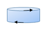so the polarization, regarded as generating a surface charge density, is equivalent to a disc of positive charge, and one of negative charge, slightly displaced, rotating the same way. Far away, one disc would give a dipole magnetic field, the two together give a quadrupole field.

A simple way to see this is to think of just two equal rings, on the same axis, separated by a distance small compared with the radius, and with an (imaginary) cylindrical surface between them. Currents are going in opposite directions in the two rings. We can represent the currents equivalently by adjacent square current loops around the cylindrical surface.

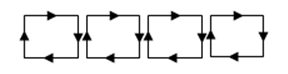
These loops of current generate a magnetic field, let's say radially inwards all around the ring. Then it will go outwards in both polar directions: a quadrupole field.

A less realistic but easy to understand scenario is to consider an infinite plate of dielectric, bounded by the planes $z = 0, z = d,$ uniformly polarized in the $z$ -direction, and moving at steady velocity in the $x$ -direction. The polarization is equivalent to two sheets of (opposite) charge on the two surfaces: when in motion, we have opposite current sheets, hence a magnetic field in the $y$ -direction between the sheets, zero outside.

This is just a taste of generalizing Maxwell’s equations to moving media, first done by Minkowski in 1908. The extended Maxwell equations are given in Landau and Lifshitz, Electrodynamics of Continuous Media, 2^nd edition, page 260. (But it’s a relativistic presentation.)

previous index next