41. Energy Flow, Maxwell's Electromagnetic Stress Tensor, Poynting's Vector
Where's the Energy?
We’ll begin with electrostatics.
First, a brief recap. The potential energy of a static continuous distribution of charge is
Where, exactly, is this energy located? It's natural to think that if a local charge density is then the energy density is locally , which could certainly be positive or negative. (We could add a tiny charge somewhere where it wouldn't significantly affect the others, then its contribution to would depend on its sign.) On the other hand, writing and integrating by parts,
so it's always positive definite, and the energy resides in the electric field.
How do we reconcile that with the fact that a positive charge in the neighborhood of a negatively equally charged object certainly has a negative potential energy, the binding energy? The point is that in claiming the energy is negative, we've ignores the energy residing in the fields of those charges even when they're far apart. Think of the energy in the distant parts of those fields: when we bring the opposite charges together, the distant fields almost cancel. True, the fields between them will reinforce, we have to do an integral over all space to find the change in field energy, but we can already see there's no obvious contradiction.
Faraday’s Picture of the Electric Field
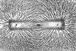 Faraday's envisioning of the electric field
undoubtedly originated with this familiar pattern of iron filings in a magnetic
field.
Faraday's envisioning of the electric field
undoubtedly originated with this familiar pattern of iron filings in a magnetic
field.
You can get a pretty good approximation to a single-charge field, a monopole, with the end of a long magnetized rod. Taking the other end of a similar magnetized rod, and putting them close (compared with rod length), the filings will delineate the field of two opposite charges. Since it was well-known that both the electrostatic field from a localized charge, and the magnetic field from the end of a long bar magnet are radial and strength decreases as the inverse square of distance, and of course fields from two charges (or two magnetic poles) add linearly, it follows that the field lines for the two cases must look the same.
So how can we picture the force acting between two charges using these field lines? This was Faraday’s great insight into the
physical reality of the field. To see it, first draw the lines for unlike
charges. As you do work dragging the
charges apart, you're stretching the
field lines -- so they behave as if they're elastic, they want to be as short
as possible. 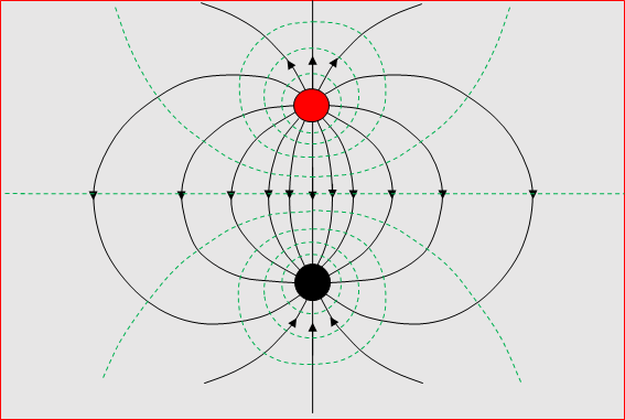 On the other hand, they don't all get in line between the poles --
they seem to be pushing each other sideways.
On the other hand, they don't all get in line between the poles --
they seem to be pushing each other sideways.
Remember that at the time, light was envisioned as a wave in some elastic medium, the ether. The electric and magnetic fields were thought to represent tensions and stresses in this mediumthat was Faraday’s picture. We don't think about it in quite that way anymore, for one thing such a traditional elastic medium would have a definite rest frameit was called the etherwhich we now know is not the case. But many ideas prove to be independent of the model: the field does contain stresses, it does exert pressures, Maxwell's stress tensor, which quantifies the stresses as functions of the fields, is correct, despite the lack of an ordinary material medium.
What about two positive charges?
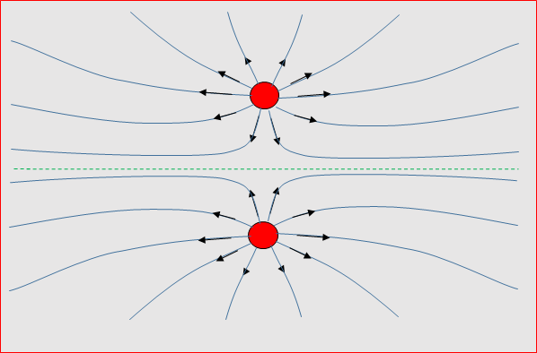 The field lines all go off to infinity: if we
push the charges closer together, that isn't particularly stretching or
compressing those lines. This time, it's
the local sideways force that's dominating the picture.
The field lines all go off to infinity: if we
push the charges closer together, that isn't particularly stretching or
compressing those lines. This time, it's
the local sideways force that's dominating the picture.
Faraday talked in these terms at a time when almost nobody took the concept of a field seriously, the standard model was action at a distance, with no further explanation thought necessary. It worked so well for gravity, after all. And, Faraday didn't know any mathematics, so he couldn't express himself in the theoretical language of the day. It was only when Maxwell read Faraday's work and figured out how to translate the ideas into differential equations that progress happened.
We’ll find that Maxwell’s analysis of the field makes clear that the force between the two charges, in both cases, is given precisely by stresses and tensions in the field across the dotted line between them. (The expressions are simplest therebut in fact any dividing boundary would work.)
Maxwell Does the Math: The Electric Stress Tensor
To quantify Faraday's ideas about the stresses in the electric fields, the tensions along lines of field and repulsions between them, Maxwell introduced the electric stress tensor.
Suppose we have some electrostatic distribution of charge in space. What is the total electrical force felt by the charge contained in a given subvolume ?
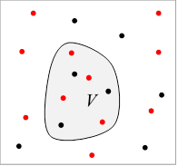
We can just write
where includes delta functions for point charges.
It doesn't matter that the electrical field is partially generated by charges within the volume, those force terms will cancel in pairs.
This total force on the charge within can be expressed purely in terms of the electric field, by writing then rearranging to write the integral as one over a divergencebecause then we can transform it into a surface integral enclosing It will then become apparent that the total force on the charge in is a combination of normal-force pressure and sideways force shear on the surface of
To see how this works, take one component of the force:
Then use (from ) to get
The integrand is the divergence of the Maxwell electric stress tensor:
Therefore, using the divergence theorem, the total force on the charge within the volume is exactly equivalent to a force on the confining surface:
that is,
As mentioned above, a simple example worth thinking through is the force between two point charges: enclose one of them by taking the bisector plane plus a hemispherical surface at infinity (which latter gives no contribution, since the integrand goes down as ). For unlike charges, the field is perpendicular to the surface, the Faraday picture is that these lines are under tension. For like charges, the electric field lines at the plane are parallel to the plane, and repelling each other sideways, again giving force in the normal direction.
Actually, this expression has to be correct integrating over any enclosing surface. The normal term is simply a pressure, equal to the energy density, giving the work needed to move the surface infinitesimally in the normal direction. The other term includes force along the surface, to be discussed later.
Energy Density and Energy Flow: Poynting's Vector
Field Only
At this point, we’ll generalize from electrostatics to time dependent electromagnetic fields. In this section, we are considering fields and charges in a vacuum. In the following two sections, we look at energy flow in materials.
We found the expression for energy density in an electric field (above), and, earlier, we found that in a magnetic field. We will assume these expressions remain valid in a general time-dependent electromagnetic problem, where now the local energy densities ebb and flow. As shown below, Poynting proved that the vector measures the local energy flow rate, so a simple conservation equation, analogous to the charge conservation equation could be written for the total field energy density.
Here's how he did it: denote the local energy density in the field by
The local rate of change of this energy density is
Exercise: Check that last line, using the notation. (Easier to work backwards.)
The vector is the Poynting vector, measuring energy flow. It can be put in integral form to find the rate of change in a fixed volume:
Field + Charges
But if there are charged particles in the volume, field energy can be expended working on these charges (or the other way round).
To include this possibility, suppose there is a current density so the electric field is doing work on the charges equal to
With these currents present, from Maxwell’s equation so the rate of change of local electrical field energy must be
That is, the rate at which the field is working on the moving charges is the rate at which the field itself is losing energy (of course!).
Remember the force on the particles from the magnetic field is perpendicular to the velocity, so does no work, therefore exchanges no energy.
This means the total rate of change of energy in the volume (meaning field energy plus particle energy) is still given by integrating the Poynting vector over the boundary surface (assuming there is zero particle flow across the surface).
Momentum Conservation: Maxwell's Stress Tensor Again
Although the Lorentz force does no work, it does of course change the momentum of a charged particle: so there must be a transfer of momentum from the field to the particle, analogous to the energy exchange discussed above. (We're talking here about the mechanical momentum of the particle, good old mass times velocity: we mention this because in the Lagrangian formulation of E&M, there is a variable called the canonical momentum, which includes a field term. Note also that we haven't got to special relativity yet, so these are nonrelativistic particles. We'll find later that the generalization to relativistic particles is straightforward.)
Anyway, for a collection of charged particles and fields in a volume (and assuming no particles cross the volume boundary)
We're going to show that this rate of change of mechanical momentum comes from the fields, so we need to express the right-hand side purely in terms of fields. Inserting
we find
But what is happening to the momentum in the fields themselves? We need to think: we know from the section above that energy flow across a surface is given by the Poynting vector, and we know that the energy-momentum relationship for a plane wave is the same as for a photon, suggesting that the local momentum flow rate is Therefore the local momentum density, since electromagnetic flows are at the speed of light, must be
Assuming this hand-waving is correct, the rate of change of total momentum within the volume is
Notice that the term appears in both the rate of change of mechanical momentum and that of field momentum, but with opposite signs, it is therefore momentum transfer between particles and fields within the volume. Our aim here is to find the total rate of change of momentum within the volume as an integral over a divergence, so that it can be transformed to a surface integral over the boundary (we are assuming that no particles are crossing the boundary).
Adding together the mechanical momentum and the field momentum, and writing as we find
where we've also added the identically zero term to emphasize the electric-magnetic symmetry.
As we've said, the aim is to write this integrand as a divergence. It turns out to be the divergence of a tensoras it must, since it's a vector. It is a straightforward exercise to show that
The expression in parentheses on the right is the electrical component of the Maxwell stress tensor:
(Note: We found the electrical part of this tensor earlier in calculating the total electrical force on charges enclosed by a specified surface, expressed as a force acting on the surface. Since force is rate of change of momentum, that same expression gives the electrical field contribution to the rate of change of momentum, or momentum flow across the bounding surface.)
Evidently, the same vector identities work for the mathematically identical magnetic components, so we get:
(Here we've used the summation convention: repeated suffixes are summed over.)
That is, the component of Maxwell's stress tensor gives the local flow rate of the -component of momentum density through a plane having normal in the -direction. This is exactly the same physically as the stress tensor used in discussing stresses and strains in continuous media in classical mechanics.