44.  Symmetries and the Dirac Monopole

    Michael Fowler, UVa

Transformation of Fields and Sources: Rotation, Reflection, Time Reversal

(Jackson 6.10)

As we reviewed in the math bootcamp, in rotations, position vectors transform as

$x_i{}^{\prime }=R_{ij}{x}_{j,}$ 

using the summation convention (double appearance of suffix in one expression implies summation, here over 1,2,3).  An ordinary rotation is termed an orthogonal transformation, its inverse is its transpose (which has the same determinant), consequently the square of the determinant ${\left|R\right|}^2=1.$  The determinant is itself equal to one for a rotation, but its square is still one even if a reflection is included, such as $x^{\prime }=x,y^{\prime }=y,z^{\prime }=-z$, sometimes termed an improper rotation.  This reflection in the $xy$ plane can be combined with a $\pi$-rotation in that plane to get spatial inversion, having matrix representation $R_{ij}=-{\delta }_{ij}.$    

Ordinary vectors, such as position, velocity, and acceleration are of course reversed under spatial inversion, but this is not true of the angular momentum vector $\overrightarrow{x}\times \overrightarrow{p},$ which doesn't change. 

Vectors that do not change sign under spatial inversion are called pseudovectors or axial vectors.  In this context, ordinary vectors are sometimes referred to as polar vectors.

Scalars, such as $\overrightarrow{a}\cdot \overrightarrow{b}$ or $\overrightarrow{\nabla }\cdot \overrightarrow{E}$ (the vectors being polar) do not change sign under spatial inversion, but the triple product of polar vectors $\overrightarrow{a}\cdot \left(\overrightarrow{b}\times \overrightarrow{c}\right)$ does, so it is termed a pseudoscalar.

Recall that in transforming a tensor there is one factor of $R_{ij}$ for each suffix, so a second-order tensor, such as Maxwell's stress tensor, will transform as $T_{ij}{}^{\prime }=R_{im}{R}_{jn}{T}_{mn},$ and similarly for higher orders.  A tensor of order $N$ transforms under spatial inversion with a factor ${\left(-1\right)}^N,$ a pseudotensor ${\left(-1\right)}^{N+1}.$ 

Time Reversal Invariance

The laws of classical (and almost all of quantum) physics are the same if time is reversed. If you have a movie of planets going around a sun, and play it backwards, it will still show a system following the laws of physics.  Under time reversal, ${\overrightarrow{x}}^{\prime }=\overrightarrow{x},{\overrightarrow{p}}^{\prime }=-\overrightarrow{p}$ so angular momentum ${\overrightarrow{L}}^{\prime }=-\overrightarrow{L}:$ the planets go the other way, but still obey Newton's equation, ${\dot{\overrightarrow{p}}}^{\prime }=-\overrightarrow{\nabla }U\left({\overrightarrow{x}}^{\prime }\right):$ forces do not change sign under time reversal (think of force as rate of change of momentum), nor do accelerations$—$the planets still circle the sun.

Electromagnetic Quantities

Just as velocity is odd under time reversal, so is current $q\overrightarrow{v}.$ (We assume, of course, that charge doesn't change under any of the transformations discussed here. There is no evidence to the contrary.)

Slightly less evident is that magnetic fields and magnetization must be odd under time reversal, since they are generated by circulating currents (or spin, which is an angular momentum).

The Poynting vector is odd under time reversal (it's an energy flow).

Charge stays the same, so the electric field, force per unit charge, is invariant under time reversal.

Consider $\overrightarrow{\nabla }\times \overrightarrow{E}+\dot{\overrightarrow{B}}=0.$  Under time reversal, both terms stay the same. ( $\overrightarrow{B}\to -\overrightarrow{B},$ so $\dot{\overrightarrow{B}}\to \dot{\overrightarrow{B}}.$ )

Under spatial inversion, both terms don’t change sign.

(Keep in mind the picture of the magnetic field from a current loop.  Either spatial inversion or time reversal will send the current the other way.)  Using the jargon, the current is a polar vector, meaning it reverses under spatial inversion, as an ordinary vector, like position, would. 

The bottom line is:

 $\rho$ is a scalar, and even under time reversal.

$\overrightarrow{J}$ is a vector, odd under both space and time reversal.

$\overrightarrow{E}$ is a vector, odd under space inversion, even under time reversal (as also are $\overrightarrow{D},\overrightarrow{P}$ ).

$\overrightarrow{B}$ is a pseudovector, even under space reversal, odd under time reversal (as are $\overrightarrow{H},\overrightarrow{M}$ ).

If magnetic monopoles exist, then from $\overrightarrow{\nabla }\cdot \overrightarrow{B}={\rho }_M,$ the monopole density ${\rho }_M$ would be a pseudoscalar, and odd under time reversal.  (Just like the "pole" at the end of a bar magnet!)

If the Maxwell stress tensor is dotted into an ordinary vector, it yields a force, so it is even under both space inversion and time reversal.

One reason these properties are worth reviewing is that for continuous media systems with both electric and magnetic fields present, where we have no complete microscopic theory, it is often fruitful to develop a phenomenological theory$—$Landau was very good at this.  Demanding your equations obey certain symmetries, such as parity invariance (under space inversion) constrains the products of fields that can appear in higher-order terms.

In particle physics, the pion is pseudoscalar, so can only link to an axial current.  Symmetry considerations greatly constrain possible models of elementary particle interaction.

Furthermore, these symmetries are very important in modern condensed matter quantum theories, such as the quantum Hall effect and topological insulators.

The Dirac Magnetic Monopole

(Jackson 6.11, 6.12)

We'll begin with the motion of a particle of mass $m,$ charge $e$ in the magnetic field of a monopole (taken fixed) of strength $g,$ meaning magnetic field

$\overrightarrow{B}\left(\overrightarrow{r}\right)=\frac{g\widehat{\overrightarrow{r}}}{4\pi r^2}.$ 

The equation of motion is:

$m\ddot{\overrightarrow{r}}=e\dot{\overrightarrow{r}}\times \overrightarrow{B}.$

Question: The field is spherically symmetric: does that mean angular momentum is conserved?

(Remember, Noether's theorem says each symmetry of a system has a corresponding conserved quantity.)

Well, here it looks like it can't possibly be: the force has nonzero torque about the center!

In fact, we can rather easily find the rate of change of orbital angular momentum:

$\begin{array}{c}\frac{d}{dt}\left(\overrightarrow{r}\times m\dot{\overrightarrow{r}}\right)=\overrightarrow{r}\times m\ddot{\overrightarrow{r}}\\ =\frac{eg}{4\pi r^2}\widehat{\overrightarrow{r}}\times \left(\dot{\overrightarrow{r}}\times \overrightarrow{r}\right)\\ =\frac{d}{dt}\left(\frac{eg}{4\pi }\widehat{\overrightarrow{r}}\right).\end{array}$ 

Exercise:  Check this result.

This suggests defining the total angular momentum as

$\overrightarrow{L}=\overrightarrow{r}\times m\dot{\overrightarrow{r}}-\frac{eg}{4\pi }\widehat{\overrightarrow{r}},$ 

which is a conserved quantity, so this is how Noether's theorem is satisfied? What does it mean?

We've established that a system with non-zero electric and magnetic fields will have a momentum density$—$the explanation has to be that this extra term is a field angular momentum density.

To check, recall the Poynting vector gives local field momentum density ${\mu }_0^{-1}\left(\overrightarrow{E}\times \overrightarrow{B}\right)/c^2,$ so the field angular momentum will be 

${\overrightarrow{L}}_{\text{field}}={\mu }_0^{-1}{\displaystyle \int d^{3}r\left[\overrightarrow{r}\times \left(\overrightarrow{E}\times \overrightarrow{B}\right)\right]}/c^2.$ 

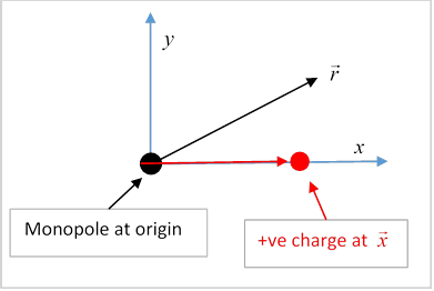
For the electric charge at $\overrightarrow{x},$ say, the electric field is $\overrightarrow{E}\left(\overrightarrow{r}\right)=\frac{e}{4\pi {\epsilon }_0}\frac{\overrightarrow{r}-\overrightarrow{x}}{{\left|\overrightarrow{r}-\overrightarrow{x}\right|}^3}.$ 

The (monopole at the origin) magnetic field is  $\overrightarrow{B}\left(\overrightarrow{r}\right)=\frac{g\widehat{\overrightarrow{r}}}{4\pi r^2}.$ 

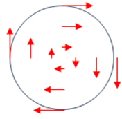
Exercise:  sketch the momentum density for this combination of fields, and convince yourself that the field angular momentum vector must point along the line from the pole to the charge.

The field angular momentum integral doesn't look too easy (try plotting it for a given separation), but the trick is to avoid messing with the expression for electric field.  That is, we write it as

$\begin{array}{c}{\overrightarrow{L}}_{\text{field}}=\frac{g}{4\pi {\mu }_0}{\displaystyle \int d^{3}r\left[\overrightarrow{r}\times \left(\overrightarrow{E}\times \frac{\widehat{\overrightarrow{r}}}{r^2}\right)\right]}/c^2\\ =\frac{g}{4\pi {\mu }_0}{\displaystyle \int d^{3}r\left[\frac{\overrightarrow{E}-\overrightarrow{r}\left(\overrightarrow{r}\cdot \overrightarrow{E}\right)}{r}\right]}/c^2\\ =\frac{g}{4\pi {\mu }_0}{\displaystyle \int d^{3}r\left[\overrightarrow{E}\cdot \overrightarrow{\nabla }\widehat{\overrightarrow{r}}\right]}/c^2=-\frac{g}{4\pi {\mu }_0}{\displaystyle \int d^{3}r\left[\widehat{\overrightarrow{r}}\overrightarrow{\nabla }\cdot \overrightarrow{E}\right]}/c^2\\ =-\frac{eg}{4\pi {\mu }_0{\epsilon }_0{c}^2}\widehat{\overrightarrow{x}}=-\frac{eg}{4\pi }\widehat{\overrightarrow{x}},\end{array}$

where we used $\overrightarrow{\nabla }\widehat{\overrightarrow{r}}=\overrightarrow{\nabla }\frac{\overrightarrow{r}}{r}=\frac{{\delta }_{ij}-{\widehat{r}}_i{\widehat{r}}_j}{r}.$  So it checks: and notice this angular momentum will be in the field even if both particles are at rest.  So conservation of total angular momentum is OK.

Important:  Notice that the total field angular momentum does not depend on the distance between the monopole and the charge.

Dirac Quantization

This field angular momentum result has dramatic consequences in quantum mechanics, where one of the most fundamental assumptions is the quantization of angular momentum$—$that's how the Bohr atom began.  An electron at rest in the magnetic field of a monopole at rest has nonzero field angular momentum, which must be quantized, possibly in half units,

$\frac{eg}{4\pi }=\frac{n\hslash }{2},$  with $n$ an integer$—$and the distance apart doesn't matter. 

So if there is one monopole in the universe, all electric charges must be multiples of some basic unit of charge!  This is the first explanation of why all electrons have exactly the same charge, and other particles have multiples of it (including negative multiples, of course).

For $n=1$ or $2,$ the monopole magnetic coupling strength is very large, so if such particles exist, they should be easy to detect.  But so far, no luck…

Exercise: Making the simplest assumption, that $eg/4\pi =\hslash ,$ show that Jackson’s equation (6.156) for the change in angular momentum of a charge scattered by a monopole follows immediately.

Monopole Vector Potential

The field is spherically symmetric, and decreasing as the inverse square of radial distance. If we can find an expression for the vector potential on a spherical surface, the same expression will work everywhere with a $\left(1/r\right)$ factor.  (Of course, the vector potential is not unique, we'll see how that works here later.)

So we need to construct a vector field on the surface of the sphere with a constant (outward pointing) curl. 

We know how to do that on a plane: a steadily rotating object has a velocity field with constant perpendicular curl, that is, a field $\left(0,r\widehat{\overrightarrow{\varphi }}\right).$ Let's take a vector looking like that near the north pole of the sphere.  In fact, we can consistently take the $\overrightarrow{A}$ field to be in the $\widehat{\overrightarrow{\varphi }}$ direction, and its magnitude can be found by  integrating around a line of constant latitude, a length $2\pi r\sin \theta ,$ 

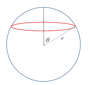
this integral must equal the field $\overrightarrow{\nabla }\times \overrightarrow{A}\cdot \widehat{\overrightarrow{n}}=\overrightarrow{B}\cdot \widehat{\overrightarrow{n}}$ over the total globe surface north of that latitude, that is, $g/4\pi r^2$ over  an area $2\pi r^2\left(1-\cos \theta \right).$ Thus

$\begin{array}{c}2\pi r\sin \theta A\left(r,\theta \right)=\frac{1}{2}g\left(1-\cos \theta \right),\\ \overrightarrow{A}\left(r,\theta \right)=\frac{g\left(1-\cos \theta \right)}{4\pi r\sin \theta }\overrightarrow{\varphi }.\end{array}$ 

We can now see that things go bad as we approach the south pole. What happened?

Well, actually, a monopole as we've defined it cannot have a vector potential valid throughout space, because for a monopole obviously $\overrightarrow{\nabla }\cdot \overrightarrow{B}\ne 0$ at the origin, but $\overrightarrow{\nabla }\cdot \overrightarrow{\nabla }\times \overrightarrow{A}\equiv 0$ everywhere, for a well-defined $\overrightarrow{A}.$ So what does the $\overrightarrow{A}\left(r,\theta \right)$ we've constructed above describe?  A clue can be found by taking a small circular contour around the south pole. We've found the vector potential on that contour by taking a spanning surface covering almost the whole surface of the globe.  But what if we'd taken just the tiny circular surface including the south pole? We have to get the same result$—$but we don’t.

Dirac resolved this by postulating that the monopole was actually the end of an extremely thin solenoid, a tube of magnetic flux, whose other end, possible far away, was another monopole, but of opposite sign. Then he had to figure out how this string could be undetectable$—$but for that we need quantum mechanics.

Recall that the way a magnetic field is introduced in finding the motion of a nonrelativistic charged particle in classical mechanics is to write the kinetic energy term as

$E_{\text{kin}}=\left(1/2m\right){\left(\overrightarrow{p}-e\overrightarrow{A}\right)}^2,$ 

where $\overrightarrow{A}$ is the vector potential.  In quantum mechanics, $\overrightarrow{p}\to -i\hslash \overrightarrow{\nabla }$.

 

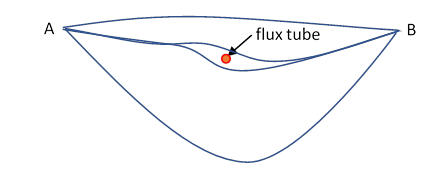
Using Feynman's approach, the probability amplitude for finding an electron at a point B given that earlier it was at  A  can be expressed as a sum over all possible paths from A to B, with the appropriate phase change along that path. Suppose we are far away from the monopole, so that its magnetic field is negligible$—$but the flux tube passes through our region. Since it carries total magnetic field $g$, we must have

        ${\displaystyle \oint \overrightarrow{A}\cdot d\overrightarrow{l}=g}$ 

for any contour going once around the flux tube.  Now the phase of the wave function along a path is given by $e^{i\left(\overrightarrow{p}-e\overrightarrow{A}\right)\cdot \overrightarrow{x}/\hslash }.$ Consider two paths that are identical except that in the immediate vicinity of the flux tube they pass it on opposite sides. The presence of the flux tube will therefore change the relative phase between the two paths shown by ${\displaystyle \oint e\overrightarrow{A}\cdot d\overrightarrow{l}/\hslash }=ge/\hslash$ taken around the loop formed by the difference between the two paths.  The presence of the flux tube will therefore affect the propagation of the electron unless $ge/\hslash =2n\pi .$ But this is precisely the condition demanded by the quantization of angular momentum of an electron close to a monopole.  So, if that is satisfied, the string makes no detectable impact on the motion of charged particles.

Real Monopoles?

It turns out that something very close to a Dirac string occurs in certain superconductors (see next section), and also many particle theorists think there might be monopoles out there somewhere, but in the modern view, the magnetic monopole has lost its tail.  The string came from Dirac's analysis, which was purely in terms of the gauge theory of electromagnetism, and was an inevitable result of the gauge field, which has a $U\left(1\right)$ symmetry, equivalent to rotations in a plane.  A two-dimensional vector field with this symmetry cannot be continuously defined everywhere on the sphere, that's why the Dirac solenoid string was introduced.  But we now know that the electromagnetic field is one of a family of fields, including the weak interactions, and by using Maxwell's equations we are assuming a low energy limit. However, close enough to the monopole, this approximation is no longer valid, we need to include more fields, and then it turns out that the gauge vector field is no longer two-dimensional$—$essentially, it can point out of the plane.  This gets us off the hook without the string.  If you're curious to see details on constructing a monopole in this way without a string, click here.

The Magnetic Flux Quantum

In the simplest possible nontrivial solution of $ge/\hslash =2n\pi ,$ taking $n=1,$ the total flux going down the tube is $\varphi =h/e.$  Confusingly, there is another flux quantum, $h/2e,$ that is important in superconductivity.  Usually, superconductivity and magnetic fields don't mix well.  For one class of materials, known as type II superconductors, a magnetic field will penetrate the superconductor with an array of parallel strings, the material remaining superconducting away from these strings. In the superconductor, the electrons have what amounts to a macroscopic wave function, except that they are bound in pairs, so the effective particle charge is $2e.$ For the wave function to match up on going round a flux tube, then, it must have total flux some multiple of $h/2e.$  It turns out that tubes with a multiple of this number are unstable, and break up into smaller tubes carrying this quantum.  This quantization was first observed by Deaver and Fairbank (our own Bascom Deaver).

How Real is the Vector Potential?

(Experiment in Phys Rev Lett 56, 792, 1986.)  A small toroidal magnet was constructed: the magnetic field goes around the ring. It was encased in a layer of superconducting material, to ensure that no stray magnetic field reached the outside. An electron beam was directed at the ring, some went through, some outside the ring, and the interference pattern on a screen was observed. It precisely matched the theory presented above: the vector potential caused a phase difference between the electron wave going through the ring and that passing on the outside.  To ensure that the electron wave function could not reach the region where the magnetic field was nonzero, a further layer of copper was added on top of the superconductor. The point is that the nonzero vector potential had a measurable physical effect on a particle that never entered the region where the magnetic field was nonzero, and there was zero electromagnetic field energy everywhere the particle traveled.

So the moral to this story is that once quantum mechanics comes in, the electric and magnetic fields are not the whole story. The vector potential is not merely a convenient mathematical device for solving equations, it can change wave functions even in regions where the fields are zero. For more on this, click here.

previous  index  next