47.  Frequency Dispersion in Dielectrics and Conductors

    Michael Fowler, UVa

(Jackson sections 7.5 A, B, C.)

What Does This Mean?

"Frequency dispersion" means the permittivity (a.k.a. dielectric constant) is a function of frequency: $\epsilon =\epsilon \left(\omega \right)$. Think of light going through a prism: different colors are refracted through different angles, the refractive index $n=\sqrt{\epsilon /{\epsilon }_0}$ varies, hence so does the velocity of the wave in the glass. You could say the prism disperses the colors, which it couldn't do for a constant $\epsilon$ material. Here's a more direct visualization of the  dispersion: imagine a short pulse of white light traveling through space, it will hold its shape indefinitely, but if it enters a dielectric, the different colors it's made up of will travel at different speeds, and it will become a multicolored spreading blob. That's dispersion.

Simple Model for $\epsilon \left(\omega \right)$ 

Begin with a slightly generalized Lorentz molecule, an electron bound by a harmonic force, and having its motion damped:

$m\left[\ddot{\overrightarrow{x}}+\gamma \dot{\overrightarrow{x}}+{\omega }_0{}^2\overrightarrow{x}\right]=-e\overrightarrow{E}\left(\overrightarrow{x},t\right).$ 

Assuming the external field has time variation $e^{-i\omega t},$ the dipole moment from this one electron is 

$\overrightarrow{p}=-e\overrightarrow{x}=\frac{e^2}{m\left({\omega }_0{}^2-{\omega }^2-i\gamma \omega \right)}\overrightarrow{E},$ 

the familiar formula for a driven damped oscillator (in steady oscillation, after initial transients have died away).

Now suppose these bound electrons (the simplest possible model for an atom!) have number density $N$ in the dielectric medium, so they will contribute polarization of strength $\overrightarrow{P}=N\overrightarrow{p}.$ 

 From $\overrightarrow{D}=\epsilon \overrightarrow{E}={\epsilon }_0\overrightarrow{E}+\overrightarrow{P},$ we find for this simple model

$$\frac{\epsilon \left(\omega \right)}{{\epsilon }_0}=1+\frac{N{e}^2}{{\epsilon }_{0}m\left({\omega }_0^2-{\omega }^2-i\gamma \omega \right)}.$$  To better approximate a real solid, take in each molecule oscillating electrons with different natural frequencies and damping, so the dielectric response becomes

$$\frac{\epsilon \left(\omega \right)}{{\epsilon }_0}=1+\frac{N{e}^2}{{\epsilon }_{0}m}{\displaystyle \sum _j\frac{f_j}{{\omega }_j{}^2-{\omega }^2-i{\gamma }_j\omega }.}$$  Here $f_j$ is the number of electrons in a molecule with parameters ${\omega }_j,{\gamma }_j,$ and now $N$ is the number of molecules in unit volume.  Generally, these oscillations are lightly damped, ${\gamma }_j$ is small, so $\epsilon \left(\omega \right)$ has a very small imaginary part except very close to one of the ${\omega }_j$ 's.

The oscillator strengths satisfy a sum rule, ${\displaystyle \sum _j{f}_j=1.}$

To derive this properly needs quantum mechanics, but we can see how it comes about in our simple classical model by looking at the $\omega \to \infty$ limit, where the electrons are effectively free, equivalent to a plasma. We find $\epsilon \left(\omega \right)$ for a plasma below, that gives the sum rule.

The model has damped oscillators, so energy is being absorbed from the light wave, and the wave number $k$ must therefore be complex, to include attenuation.

Since $-{\omega }^2$ appears in the denominator, $\epsilon \left(\omega \right)$ tends to increase with $\omega ,$ at least for low $\omega ,$ this is termed normal dispersion.  Near the resonance frequencies ${\omega }_j,$ there are rapid changes, and there will be regions where $\epsilon \left(\omega \right)$ is decreasing, called anomalous dispersion. 

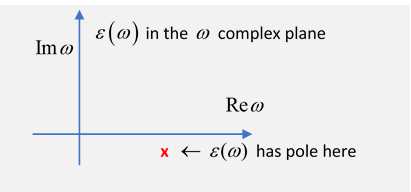
It's worthwhile thinking of $\epsilon \left(\omega \right)$ as the real axis value of a function of a complex variable, $\epsilon \left(z\right).$ 

Near a resonance, there is a pole in the lower half plane near the real axis, a root of the equation ${\omega }_0^2-{\omega }^2-i\gamma \omega =0,$ at $\omega =-\frac{1}{2}i\gamma +{\nu }_0,{\nu }_0^2={\omega }_0^2-\frac{1}{4}{\gamma }^2.$ 

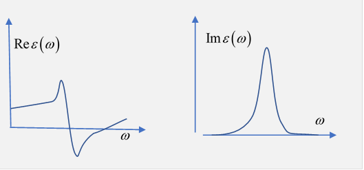
Exercise:  sketch the general shape of $\mathrm{Re}\epsilon \left(\omega \right),\mathrm{Im}\epsilon \left(\omega \right)$ on the real axis, close to the pole.

 

Answer:

Close enough to the resonances, energy will be strongly absorbed from the field and fed to the damping mechanism $\gamma$  (probably generating phonons, meaning heat, essentially).  The wave number has an imaginary part, 

$k=\beta +\frac{1}{2}i\alpha ,$ 

we put in the $\frac{1}{2}$ because the wave then has intensity going as $e^{-\alpha z}$: $\alpha$ is called the attenuation coefficient.   To express it in terms of the complex dielectric function $\epsilon \left(\omega \right),$ we use

$$\frac{\omega }{k}=\frac{c}{n}=\frac{c}{\sqrt{\epsilon /{\epsilon }_0}}$$ so

$$k^2=\frac{{\omega }^2}{c^2}\frac{\epsilon \left(\omega \right)}{{\epsilon }_0}$$  and matching real and imaginary parts of the two sides of the equation,

$$\begin{array}{l}{\beta }^2-\frac{{\alpha }^2}{4}=\frac{{\omega }^2}{c^2}\mathrm{Re}\epsilon /{\epsilon }_0,\\ \beta \alpha =\frac{{\omega }^2}{c^2}\mathrm{Im}\epsilon /{\epsilon }_0.\end{array}$$  For the usual situation of not too strong absorption, $\alpha \ll \beta ,$ and

$$\alpha \cong \frac{\mathrm{Im}\epsilon \left(\omega \right)}{\mathrm{Re}\epsilon \left(\omega \right)}\beta ,$$  Notation:  We're following Jackson here. A more common notation is to write

$\epsilon =\mathrm{Re}\epsilon +i\mathrm{Im}\epsilon ={\epsilon }^{\prime }+i{\epsilon }^{″}.$

Typically $\mathrm{Re}\epsilon \left(\omega \right)$ is of order one$—$and notice from the graph that it is decreasing as a function of frequency in the immediate neighborhood of the resonance.

Low Frequency Behavior and Electrical Conductivity

If we allow for the possibility of free electrons in the dielectric, then we'll get an extra term in the $\overrightarrow{\nabla }\times \overrightarrow{H}$ equation from the consequent macroscopic free electron current:

$$\overrightarrow{\nabla }\times \overrightarrow{H}=\frac{\partial \overrightarrow{D}}{\partial t}+\overrightarrow{J}.$$  Using Ohm's law $\overrightarrow{J}=\sigma \overrightarrow{E}$ and taking single frequency time dependence, with ${\epsilon }_{\text{b}}\left(\omega \right)$ being the contribution to the permittivity from the bound electrons,

$$\overrightarrow{\nabla }\times \overrightarrow{H}=-i\omega \left({\epsilon }_{\text{b}}\left(\omega \right)+i\frac{\sigma }{\omega }\right)\overrightarrow{E},$$  (that last term just being $\sigma \overrightarrow{E},$ of course!)

In other words, this generalizes the permittivity to include an imaginary term from the free electrons,

$$\epsilon \left(\omega \right)={\epsilon }_{\text{b}}\left(\omega \right)+i\frac{\sigma }{\omega }.$$  This imaginary term will naturally cause attenuation of electromagnetic waves: it's the conductivity, Ohm's law, indicating that energy is being removed from the oscillating electric field and converted into heat.  (And, we're assuming $\sigma$ is independent of frequency, a good approximation over a wide frequency range for, say, copper, but for an actual sample of material the skin effect will give a frequency-dependent effective resistance$—$we'll discuss this later.)

To connect with the previous analysis in terms of oscillating bound electrons, we had (adding b for bound)

$$\frac{{\epsilon }_b\left(\omega \right)}{{\epsilon }_0}=1+\frac{N{e}^2}{{\epsilon }_{0}m}{\displaystyle \sum _j\frac{f_j}{{\omega }_j{}^2-{\omega }^2-i{\gamma }_j\omega }}$$  and the free electrons correspond to an extra contribution having ${\omega }_j=0,{\gamma }_j={\gamma }_0$, meaning not actually bound (no “springs”), but still (for nonzero applied frequency) oscillating backwards and forwards (driven by the electric field), generally over a bigger range, and with damping ${\gamma }_0,$ so in total:

$$\epsilon \left(\omega \right)={\epsilon }_b\left(\omega \right)+i\frac{N{e}^2{f}_0}{m\omega \left({\gamma }_0-i\omega \right)}.$$  This means that for low frequencies, the free electrons are the important contribution to the permittivity,

$$\epsilon \left(\omega \right)\approx i\frac{N{e}^2{f}_0}{m\omega {\gamma }_0},$$

Comparing the two equations for $\epsilon \left(\omega \right),$ the conductivity is

$$\sigma \left(\omega \right)=\frac{f_{0}N{e}^2}{m\left({\gamma }_0-i\omega \right)},$$  Hence at low frequency

$\epsilon \left(\omega \right)\approx i\sigma /\omega ,$

 putting this with $\omega =vk=\left(1/\sqrt{\epsilon }\right)k$ we have

$k^2=i\sigma \omega .$ 

 If we restore the magnetic permeability $\mu ,$ which we’ve been taking as unity, this gives the skin depth equation we discussed in lecture 37,  for penetration of an electromagnetic wave into a conductor.

It turns out that experimentally, for good metals, the conductivity is almost independent of frequency from DC up to microwaves $\left(\omega \sim {10}^{13}\right),$ which gives a measure of ${\gamma }_0$: it also means that over this wide frequency range, we can safely ignore the $-i\omega ,$ and take

$\sigma =f_{0}N{e}^2/m{\gamma }_0.$

 (The numbers, from Jackson, for copper: $\sigma \cong 6\times {10}^7,$ $N\simeq 8\times {10}^{28}$ atoms/m³, so ${\gamma }_0/f_0\simeq 4\times {10}^{13}{\text{ s}}^{-1}.$ We assume $f_0\sim 1.$ )

Impedance for a Metal Reflector

The discussion above, and the closely related analysis of skin depth in lecture 37, can equally be written in terms of the impedance $Z.$  For a nonmagnetic metal,

$$Z=\sqrt{\frac{{\mu }_0}{{\epsilon }_{\text{b}}+\left(i\sigma /\omega \right)}}\approx \sqrt{\frac{{\mu }_0\omega }{i\sigma }}$$

at low frequencies (meaning $\omega \le {10}^{13}$ for copper, far infrared).  At these frequencies $Z\ll 1$ so the refractive index $n\gg 1,$ meaning that a wave coming in from almost any direction will be refracted close to the normal on entering the metal.

The details of the wave inside the metal were discussed in lecture 37, the wave induces currents and hence heat production, so the wave vector is complex to represent the attenuation, in fact $k^2=i\mu \sigma \omega ,$ or $k=\pm \left(1+i\right)\sqrt{\frac{{\mu }_0\sigma \omega }{2}}.$ 

The decay length

$$\delta =\sqrt{\frac{2}{{\mu }_0\sigma \omega }}$$

  is called the “skin depth”.

For a wave traveling in the $z$-direction, entering the metal normally, we take the magnetic field in the conductor to be the real part of

$H_x\left(z,t\right)=H_0{e}^{-z/\delta }{e}^{iz/\delta -i\omega t}.$ 

From $\overrightarrow{\nabla }\times \overrightarrow{H}=\overrightarrow{j}=\sigma \overrightarrow{E},$ there is an accompanying electric field:

$\begin{array}{c}{E}_y=\frac{1}{\sigma }\frac{d{H}_x}{dz}=\frac{-1+i}{\sigma \delta }{H}_{0x}{e}^{-z/\delta }{e}^{iz/\delta -i\omega t}\\ =\frac{-1+i}{\sqrt{2\sigma /{\mu }_0\omega }}{H}_{0x}{e}^{-z/\delta }{e}^{iz/\delta -i\omega t}\\ =Z{H}_{0x}{e}^{-z/\delta }{e}^{iz/\delta -i\omega t}.\end{array}$ 

So, thanks to the high conductivity and consequent low impedance, the electric field inside the metal is small compared to the magnetic field from the incoming wave.

Again from lecture 37, the local heat generation $P_{\text{resistive}}\left(z\right)=〈\overrightarrow{j}\cdot \overrightarrow{E}〉=\frac{1}{2}{\mu }_0\omega H_0^2{e}^{-2z/\delta },$ and integrating, the heat generated per unit area is $P_{\text{resistive}}=\frac{1}{4}\delta {\mu }_0\omega H_0^2.$  (See also Jackson p 355.)  If the metal is being used as a reflector, a rough measure of the fraction of energy lost to heat is the ratio of the skin depth to the wavelength of the radiation.

Here’s another derivation of the reflectivity in the infrared:  recall

$$Z=\sqrt{\frac{{\mu }_0}{{\epsilon }_{\text{b}}+\left(i\sigma /\omega \right)}}\approx \sqrt{\frac{{\mu }_0\omega }{i\sigma }}$$

and for shiny metals this is much less than one in the infrared. 

Now use

$$\frac{{E^{″}}_0}{E_0}=\frac{Z^{\prime }-Z}{Z^{\prime }+Z}$$

and take the modulus of each side squared to find the reflected intensity. Put

$$Z^{\prime }=\sqrt{\frac{{\mu }_0\omega }{i\sigma }}=\frac{1-i}{\sqrt{2}}\sqrt{\frac{{\mu }_0\omega }{\sigma }},Z=\sqrt{\frac{{\mu }_0}{{\epsilon }_0}}$$

  to get

$$R=1-\sqrt{\frac{8{\epsilon }_0\omega }{\sigma }}.$$

 See Zangwill page 611.  This is the Hagen-Rubens relation, and works well in the infrared (up to frequency around 10¹³).

Exercise:  Use $c=1/\sqrt{{\epsilon }_0{\mu }_0}$ to relate this result to the rate of energy loss to heat found above.

Drude Model

 Jackson mentions the conductivity model of Drude, which was pre-quantum mechanics, basically a pinball machine picture, the balls rolling downhill, hitting pegs inelastically, etc. 

Nowadays, conductivity is well understood, and quantum mechanics plays a crucial role.  The relevant electron velocities are not given by the energy scale $kT$ (as previously thought) but, thanks to the exclusion principle, by the Fermi energy, of order a hundred times larger.  The scattering is not directly from the crystal atoms (so this picture is misleading!), a perfect lattice is transparent to electrons over a wide energy range, the scattering is predominantly from phonons, quantized lattice vibrations. In fact, these two big errors in the original prequantum model more or less cancel.  We still have $\overrightarrow{J}=\sigma \overrightarrow{E},$ and we still call it the Drude model.

previous  index  next