53 From Oersted to Waveguides

Beginnings Revisited…

We began lecture 35 with the following pivotal discovery:

“In 1820, Oersted in Denmark noticed that a compass needle moved when he connected a battery to a nearby wire. This was the first clue that electricity and magnetism were related. Faraday discussed this observation with Oersted, then went on to several years of experimentation on the effect.” The rest is history: Maxwell’s study of Faraday’s experimental results led to his equations $—$ the whole theoretical edifice was a direct consequence of Oersted’s observation!

But there’s more $—$ much more: Oersted’s result was also the seed of our communications network. How did that happen?

The 1830’s saw a dramatic development of railway systems, rapidly replacing most of the existing transportation infrastructure: horse-drawn road vehicles and boats in canals, going single-digit mph. The first trains went around 16 mph, but this rapidly increased to 25 mph and beyond. Unfortunately, as speeds went up, and at the same time the expanding rail network grew in complexity, avoiding disastrous collisions took more and more effort. One initial solution was police with flags every mile or so along the lines, to signal the line was clear. Crossovers and junctions were challenging. Various optical communication devices were tried, but the clear communications winner by the 1840’s was a direct descendent of Oersted’s experiment: the telegraph.

The Telegraph

The basic idea is simple: at one station, have a battery and a switch, connected by two wires to another station, possibly miles away, where the wires loop into a coil, in other words an electromagnet, having an iron needle nearby. Closing the switch momentarily will cause the needle to move.

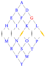
There were many fairly successful variants, including having more wires, switches and needles, the commercially successful one illustrated here, by Wheatstone and Cooke, from 1837, needed no operator training to read, but did require a six-wire connection. Two needles were energized at a time, between them they indicated a letter (G in the illustration here). This worked: it was installed on an eighteen mile stretch of rail from London to Slough, and memorably used to apprehend a murderer attempting a getaway by train in 1845. This first high tech police work got the public’s attention. However, the six-wire connectors proved to be high maintenance, and telegraphy eventually went to a simpler (but harder to interpret) two-wire system, often using the Morse code, developed in the USA.

Meanwhile in Germany, Gauss and others first installed a telegraph alongside a train line in 1835, and in the US a message was transmitted from Washington to Baltimore in 1844. The first line to the west coast opened in 1861, ending the Pony Express. The first successful trans-Atlantic cable was laid in 1866. At this point, the telegraph was no longer primarily about synchronizing trains, of course, it was transmitting all kinds of information: news, stock prices, etc. It gave the North an important advantage in the Civil War, during which thousands of miles of cable were put down.

Telegraph Physics

Thomson’s Analysis: The Law of Squares

Now for the physics. The first serious attempt to analyze the motion of a pulse of current sent down a wire was by William Thomson (Lord Kelvin) in 1855. He considered a line having resistance $R$ and capacitance $C$ per unit length, and a step voltage is applied at one end. How soon before the voltage pulse reaches some point a distance $z$ down the line? He wrote equations for the local voltage $V (z, t)$ and current $I (z, t)$ as the voltage pulse moves down the line.

Writing $Q$ for the local linear charge density, the first equation is charge conservation, the second is Ohm’s Law,

$\frac{\partial V}{\partial t} = \frac{1}{C} \frac{\partial Q}{\partial t} = - \frac{1}{C} \frac{\partial I}{\partial z}, I = \frac{E}{R} = - \frac{1}{R} \frac{\partial V}{\partial z},$

Putting these two together gives the diffusion equation

$\frac{\partial V}{\partial t} = \frac{1}{R C} \frac{\partial^{2} V}{\partial z^{2}},$

well know from the theory of heat flow.

In one dimension, the heat equation is usually written $\partial u / \partial t = k \partial^{2} u / \partial z^{2},$ and the Green’s function solution for initial $t = 0$ condition on the infinite line $u (z, 0) = δ (z)$ is

$u (z, t) = \frac{1}{\sqrt{4 π k t}} e^{- \frac{z^{2}}{4 k t}} .$

(Note this is the same as the spread of a Gaussian wave packet having zero total momentum.)

Exercise: Check this satisfies the equation.

Now, in Thomson’s case, the pulse was at one end of a wire, not the middle of an infinite wire, but the math is essentially the same, and it follows that for a strong signal to travel a distance $z$ down the cable is going to take a time of order $t \sim R C z^{2}$ (clear from a dimensional argument anyway.) This was called the Law of Squares, and received a chilly reception when Thomson presented it to telegraph engineers, who were busy planning the transatlantic cable. They had already noticed delay on much shorter lines $—$ the square of the distance was alarming. But in fact at the very lowest frequencies this law is not so far off $—$ it ignores inductance, which becomes very important as soon as attempts are made to transmit speech, needing 1,000 Hz or so signals.

Oliver Heaviside

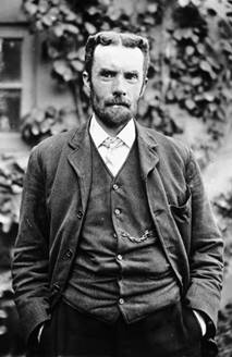
The first real progress in understanding the propagation of telegraph signals came from Oliver Heaviside. He was born in 1850, in Camden, in a rather poor part of London. As a child, he had scarlet fever, which left him almost deaf and mocked by neighborhood children, so he retreated to a back room and read a lot. He left school at age sixteen, knowing a little algebra and some trigonometry. Luckily, his aunt married Charles Wheatstone (who designed the telegraph illustrated above). In 1868 this uncle gave Heaviside a job as telegraphy clerk on a new line being opened from England to Denmark. However, in 1874 Oliver quit (having antagonized his boss) and moved back to live with his parents. He began to work in earnest on the theory of telegraphy, and in 1876 published the Telegrapher’s Equation: this began with Thomson’s analysis given above, but $—$ crucially $—$ added inductance and leakage.

The “practical men” knew from the experiments of Faraday that induction always opposed a change in current, from which they deduced (incorrectly) that induction was the enemy, and should be reduced as much as possible in a telegraph cable.

Two-Wire Representation

To see how including inductance changes signal propagation, we’ll follow a slightly simpler version of Heaviside’s analysis. The cable is modeled as two parallel wires. (The wires have small but finite thickness, and recall we found in a homework question (Jackson problem 5.29) that for general shapes of the two conductors, it's always true that $L C = μ_{0} ε_{0} .$ )

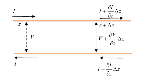
Note first that since the current intensity varies along the cable, charge is piling up or flowing away from any small section of the cable. Since it’s a capacitor, this must be changing the voltage. For capacitance $C$ per unit length, a small segment $Δ z$ has capacitance $C Δ z$ . In time $Δ t$ there is an influx of charge

$Δ Q = - \frac{\partial I}{\partial z} Δ z Δ t$

and therefore a change in voltage

$Δ V = \frac{Δ Q}{C Δ z} = - \frac{(\partial I / \partial z) Δ z Δ t}{C Δ z}$ .

That is,

$\frac{\partial V}{\partial t} = - \frac{1}{C} \frac{\partial I}{\partial z} .$

This is of course just the equation found by Thomson much earlier.

But, and Thomson missed this, the cable is also an inductance, so the changing current induces a voltage difference along the line, from the general equation $E = - L (\partial I / \partial t) .$ The small length of cable $Δ z$ has inductance $L Δ z$ , so

$\frac{\partial V}{\partial z} Δ z = - L Δ z \frac{\partial I}{\partial t},$

That is,

$\frac{\partial I}{\partial t} = - \frac{1}{L} \frac{\partial V}{\partial z} .$

Putting the two equations together,

$\frac{\partial^{2} V}{\partial t^{2}} = - \frac{1}{C} \frac{\partial}{\partial z} (\frac{\partial I}{\partial t}) = \frac{1}{L C} \frac{\partial^{2} V}{\partial z^{2}} .$

This is just a wave equation: take a solution $V = V_{0} e^{i (k z - ω t)}$ to find $ω = v k,$ with

$v^{2} = \frac{1}{L C} = \frac{1}{μ_{0} ε_{0}} = c^{2} .$

That is, provided there is vacuum, or something with essentially vacuum dielectric properties between the two cylinders, the pulse is a wave propagating at the speed of light! This is of course in complete contrast to the Law of Squares result, which ignored inductance, and can be seen as a low frequency limit.

This wave equation is the simplest version of Heaviside’s Telegrapher’s Equation, which also included resistance $R$ along the line plus leakage conductance $G$ through the material between the wires. (See the Wikipedia article for details: $R, G$ become dominant at very low frequencies $—$ at zero frequency the equations just become Ohm’s law.)

The prediction of enhanced signal speed when inductance is added led to battles between Heaviside and the “practical men” not least the chief engineer, his boss, Preece. However, it was found (counterintuitively) that indeed adding the right inductance to the cable did improve performance, sometimes substantially. This was just as well, because this same year $—$ 1876 $—$ the telephone was invented and suddenly much higher frequencies that the ponderous Morse signals became relevant.

Heaviside Reads $—$ and Understands $—$ Maxwell

After he quit his job, Heaviside (who didn’t go to college) spent his time mastering calculus and differential equations from the classic texts of the time. Next, he focused his efforts on Maxwell’s 1873 Treatise on Electricity and Magnetism. Almost no-one else was reading Maxwell’s very challenging book, which presented twenty interlocking equations relating differentials of the electric and magnetic field components. But Heaviside saw it as the key to understanding how the signal was transmitted down the cable, and with much labor and thought he reduced Maxwell’s equations to the four we know today, in terms of electric and magnetic vector fields, and the vector differential operators div, grad and curl. (Unknown to him at the time, Gibbs at Yale was following the same path. Heaviside and Gibbs deserve equal credit $—$ they joined forces in the 1880’s against mathematicians who didn’t care for vectors, the mathematicians wanted to express electromagnetic theory entirely in terms of quaternions. It didn’t catch on.)

The crucial thing Heaviside learned from studying Maxwell was that the energy is in the fields, with densities $\frac{1}{2} ε E^{2}$ and $\frac{1}{2} μ H^{2} .$ He went on to show (not in Maxwell!) that energy flow was given by the vector $\vec{E} \times \vec{H},$ but on announcing this result found that Poynting (at Cambridge) had discovered it a few months earlier. Of course, the practical men were sure the energy was flowing with the current down the wire.

The Importance of the Poynting Vector

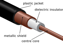
We’ll illustrate the nature of the energy flow with a specific example: the coaxial cable, patented by Heaviside himself in 1880, at which time he also presented the theory of energy transmission.

For simplicity, we’ll first look at the fields when variation along the cable is slow. (For a full analysis, see the next lecture.)

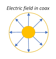
First, electric field and capacitance: see figure.

For charge density/length $λ,$ the (obviously) radial

$E = \frac{λ}{2 π ε_{0}} \frac{1}{r} .$

(Assuming for now the variation of field along the cable is small over distances of order the radius.)

As we found earlier, the capacitance per unit length is $C = \frac{Q}{V} = \frac{2 π ε_{0}}{\ln (b / a)}$ , $a, b$ being the inside and outside radii.

Now the magnetic field (remember, we’re looking in the limit where variation along the cable is slow) :

$H = \frac{I}{2 π r} .$

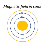
The inductance (visualize the loop formed by short circuiting one end), is $L = \frac{μ_{0}}{2 π} \ln (b / a) .$

Energy Flows in the Fields, not the Wires!

We’re now ready to track energy flow density $\vec{S}$ down the cable $—$ using the Poynting vector,

$\vec{S} = \vec{E} \times \vec{H} .$

Glancing at the electric and magnetic fields plotted above, we see immediately that the Poynting energy flow in the fields is parallel to the cable, and concentrated near the inner conductor. (To be precise, it’s at a very slight angle, some goes into the conductor, to resistance heating.)

But what about inside the wire? We know that the magnetic field inside the wire has the same pattern as outside, but decreasing linearly in strength with radius. The electric field, however, is given by Ohm’s Law, so is parallel to the cable. Therefore, the Poynting vector shows no energy transfer inside the wire parallel to the wire $—$ there is a small energy flow radially, going to heating.

As we’ll discuss in detail in the next lecture, the fields are a bit more complicated than this simple picture. In general, there are also fields parallel to the cable (but they obviously can’t add to the Poynting power flow down the cable!).

Do We Need Both Wires? The First Waveguide Analysis

Once it became clear that the energy was in the fields, and the cylindrical wire surfaces were just keeping the energy from escaping sideways, J.J. Thomson pointed out that maybe the inner wire was unnecessary. He himself had been conducting experiments on electromagnetic standing waves in cylindrical metal cans. This was the first thought of a waveguide: an electromagnetic wave sent into a metal tube might travel down the tube, being repeatedly reflected inward by the conducting walls.

Lord Rayleigh, the authority on waves, proved that in order to satisfy the boundary condition of zero parallel electric field at the conducting wall, the electric field must curve in the direction across the cable, giving a wavelength in that direction of order the diameter of the tube, and the necessary field energy would set a lower limit on the wave frequency necessary to propagate. The speed of the propagating wave would go from zero at this lowest allowed frequency, then asymptotically approaching the speed of light at high frequencies (see the next lecture for a full explanation). In 1902, R. H. Weber interpreted this speed variation by viewing the propagation down the tube as the signal traveling at the speed of light but in a zigzag path of repeated reflections. This was a correct interpretation, but in fact all this analysis was forgotten, to be rediscovered almost forty years later.

Note: In preparing this lecture I used the book Oliver Heaviside, by Paul J. Nahin, Johns Hopkins Press, 1988, 2003.

previous index next