68  Thomas Precession

    Michael Fowler, UVa

Note: Jackson covers Thomas precession twice: in 11.8 in terms of rotating frames, and covariantly in 11.11B. To match his expressions, I use Gaussian units in this lecture. I like the treatment below (from Krivoruchenko) emphasizing parallel transport, an idea central to general relativity.

Introduction: Spin-Orbit Coupling and Precession

If an atom is placed in a magnetic field, the spectral lines split up into series of close-together lines. The first explanation, before quantum mechanics, was offered by Larmor and Zeeman: imagine an electron in a circular orbit around a proton.  Now add a uniform magnetic field. If the orbit is perpendicular to the field, this adds another central force, raising or lowering the frequency depending on the direction of the circular motion.  If the field lines are parallel to the orbit, the frequency change would be negligible. This would suggest why there might be three lines, as were indeed observed in some atoms.  However, for other atoms more lines were observed, for example five.  This was termed the anomalous Zeeman effect, and was easily explained a little later with the advent of quantum mechanics: it arose from the quantization of the component of angular momentum along the field direction.

(Aside:  The Zeeman effect is used in astronomy to measure magnetic fields in stars, for example in a sunspot, and is also important in fine tuning laser Doppler slowing of atoms to catch them in a magneto optical trap at very low temperatures.)

But that wasn't the end of the story. More line splittings were observed which could only be explained by assuming the electron itself had an intrinsic angular momentum, called spin, of value $s_z=\pm \frac{1}{2}\hslash ,$ and accompanying magnetic moment $\overrightarrow{\mu }=\left(ge/2mc\right)\overrightarrow{s},g=2.$  This gave the line splittings from the magnetic field correctly, but did not properly account for the spin-orbit interaction, the energy of the electron's intrinsic magnetic moment in the field created by its orbital motion, a little circle of current.

To understand the spin-orbit interaction, we'll begin with the trivial case of an electron at the origin in a magnetic field $\overrightarrow{B}=b\widehat{\overrightarrow{z}}.$ It has a magnetic energy $U=-\overrightarrow{\mu }\cdot \overrightarrow{B},$ and will precess, $d\overrightarrow{s}/dt=\overrightarrow{\mu }\times \overrightarrow{B}$, a frequency $\omega =geB/2mc.$ 

To apply this analysis to the electron circling around the proton (we'll just do hydrogen for now), if at some instant the electron has velocity $\overrightarrow{v},$ then to leading order in $\left(v/c\right)$ the electron sees a magnetic field in its own rest frame of $\overrightarrow{B}-\left(\overrightarrow{v}/c\right)\times \overrightarrow{E},$ where $e\overrightarrow{E}=-\left(\partial V/\partial r\right)\overrightarrow{r}/r,$ $V\left(r\right)$ being the potential energy of the electron in the proton's field. 

Thus the effective orbital magnetic field is given as

$$-\left(\overrightarrow{v}/c\right)\times \overrightarrow{E}=\left(\overrightarrow{v}/c\right)\times \frac{\overrightarrow{r}}{er}\frac{\partial V}{\partial r}=-\left(\overrightarrow{r}\times m\overrightarrow{v}\right)\frac{1}{mec}\frac{1}{r}\frac{\partial V}{\partial r}.$$

 This gives an expression for the electron's total spin energy, and therefore for its precessional frequency,

$$\begin{array}{c}{U}^{\prime }=-\overrightarrow{\mu }\cdot \left(\overrightarrow{B}-\left(\overrightarrow{v}/c\right)\times \overrightarrow{E}\right)\\ =-\frac{ge}{2mc}\overrightarrow{s}\cdot \overrightarrow{B}+\frac{g}{2m^2{c}^2}\left(\overrightarrow{s}\cdot \overrightarrow{L}\right)\frac{1}{r}\frac{dV}{dr}.\end{array}$$

The problem is that this is wrong:  the $\overrightarrow{s}\cdot \overrightarrow{L}$ spin-orbit term (which, notice, is a relativistic effect) is too large by a factor of 2 compared with that observed experimentally!

(Here $g=2$ and the spin precessional frequency about the angular momentum is given by the coefficient).

So, what's wrong with the argument that led to this?

The flaw is that to find the field in the electron's rest frame, we had to do a boost from the lab frame. The spin orbit term so generated will give a precession frequency, but the problem is that the electron is constantly accelerating in a direction perpendicular to its motion, so to find the precession frequency we need to consider a series of successive incremental boosts$—$but a product of two boosts is not a pure boost, it includes some rotation, so that must be added into the rotational frequency from the energy found above, and in fact cuts the orbital contribution by a factor of two.  This result, found by Thomas in 1926, matches the experimental findings.

Dealing with a Succession of Relatively Rotated Frames

(Mostly following M. I. Krivoruchenko, arXiv:0805.1136v2[nucl-th])

Parallel Transport

As the electron circles the proton, the succession of frames in which it is momentarily at rest circle with its momentum vector.  If no magnetic field is present, the spin will as far as possible stay pointing in the same direction.

This is analogous to the famous problem of parallel transporting a vector on a spherical surface: even if the incremental transport keeps it parallel, on going around a finite closed path the arrow won't end up pointing in its original direction.  This is most easily seen by considering going around an octant, from the north pole down to the equator, with an arrow pointing along the path, then a quarter of the way around the equator, the arrow pointing now due south, then straight back up to the north pole.  On getting back, the arrow will be $\pi /2$ off from its original direction, despite being parallel transported at each step.

 A classic example, amazingly similar to Thomas precession, is Foucault's pendulum, so we'll review that first.

Foucault's Pendulum

Foucault's pendulum famously demonstrated the rotation of the Earth: it swung in a fixed plane, relative to the stars, as the Earth rotated beneath it. At colatitude $\theta$ (meaning we take the physicist's notation, $\theta =0$ at the north pole) the component of the earth's angular momentum perpendicular to the ground is $\omega \cos \theta$, and this is the observed rate of rotation of the pendulum's plane of swing.

We'll now analyze this from a slightly different point of view: in 24 hours, we see the pendulum as being transported (by the earth's rotation) along a path on the spherical surface going around one circle of latitude.  As it is moved along, we require "parallel transport", meaning that we constantly adjust it to keep it pointing in the same direction. The question is, to what extent does it turn around anyway?  We've seen that on a spherical surface, it does turn, and in fact it can be proved that it turns through an angle equal to the solid angle enclosed by the path.

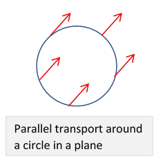
But on a flat surface, we can easily adjust the direction at each stage to keep it pointing the same way, so at the end it is still the same as at the beginning.

Notice from the diagram that on taking the arrow around a circle in a plane, the arrow always points the same way, but if we think of the angle between the circle and the path, that turns through $2\pi .$  We have to be clear which angle we're referring to.

On the surface of a sphere, parallel transport happens on moving along a segment of a great circle (meaning centered at the center of the sphere).  We could imagine going around at a constant latitude$—$not a great circle$—$as made up of many segments of great circles, but they would intersect at nonzero angles, where we'd have to adjust appropriately.  

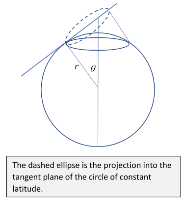
To see how much our latitudinal trip turns the arrow, let's take the sphere to have radius $r,$ then the trip has length $2\pi r\sin \theta .$ Now think about a tiny part $\left(r\sin \theta \right)\Delta \varphi$ of the path.  It's a very good approximation to take this segment to be in the tangent plane to the sphere at the point in the middle of the segment. The segment of the latitude circle projects into this plane as the end of an ellipse: the ellipse has one axis the same as the latitude circle ( $r\sin \theta$ ), the other shortened by a factor $\cos \theta$ (see figure).

The radius of curvature of the latitude circle is $r\sin \theta ,$ the local radius of curvature $r_C$ of its projection into the flat tangent plane is (larger) $r\sin \theta /\cos \theta =r\tan \theta .$ This means that as we move an arrow a small distance $ds$ along this path (which for increments is the same as the path in the local flat tangent plane) to keep it pointing in a constant direction we must rotate it through an angle  $ds/r_C=\left(ds/r\right)\cot \theta$ relative to the path. Therefore, the angle turned through in going all the way around the sphere is $2\pi r\sin \theta \left(1/r\right)\cot \theta =2\pi \cos \theta ,$ again relative to the path.  Now for a circle of latitude, on going completely around, the direction of the path relative to the fixed stars goes through $2\pi .$   So on approaching a small circle around the north pole, comparing the pendulum's direction with a fixed line in the rotating plane, the angle turned through per day approaches $2\pi$ (it's actually $2\pi \cos \theta$ ), but  relative to the fixed stars, in 24 hours the Foucault pendulum will have turned through an angle of $2\pi \left(1-\cos \theta \right),$ going to zero at the pole.

The Cone Hat Trick

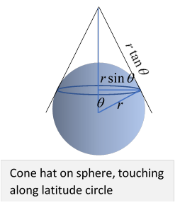
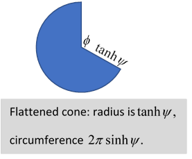
An easier way to derive this result (which we'll also use for Thomas precession) is to place a conical hat on the sphere, just touching the sphere along the line of latitude we are going to travel around.  Where they touch, the sphere and cone have a common tangent plane, so incrementally moving the arrow along the latitude, keeping its direction constant, is the same as doing it on the cone.

But, unlike the sphere, the cone can be unfurled and laid out flat. This makes it easy to see what parallel transport means: just keep the arrow pointing in the same direction in the plane. 

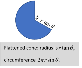
Relative to the line of latitude, then, such an arrow will have changed direction by $\varphi$ on going once around, where

$$\varphi =2\pi -\frac{2\pi r\sin \theta }{r\tan \theta }=2\pi \left(1-\cos \theta \right).$$

This agrees with our earlier finding.

Thomas Precession

The analysis of Thomas precession is remarkably similar to that above, and the cone trick works again. We're trying to track the spin direction as the electron orbits around the proton.  Remember, we are not including the precession from the magnetic field, that can be added later.  In our model, there is no physical torque on the spin, so it will be parallel transported from one frame to the next as the electron moves around.  In fact it will precess, as we've said, but it is a purely kinematical effect, arising from the successive boosts necessitated by the acceleration, the product of boosts giving rotation.  Our job is to calculate how much spin rotation comes about as a result of one orbit period.

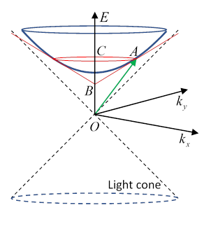
As the electron circles around the proton, it is also moving around a circle in velocity space, conveniently parametrized with rapidity $\psi .$ (Recall $\beta =\tanh \psi .$ )  Suppose at $t=0$ its 4-velocity is $\overrightarrow{OA}=\left(\gamma ,\widehat{\overrightarrow{n}}\gamma \beta \right).$  The hyperboloid (looking like a saucer) surface is the set of 4-velocities (for the three-velocity confined to the $\left(x,y\right)$ plane).

Now we imitate the analysis we just did for Foucault's pendulum.  The red circle, and red cone touching the hyperboloid along that circle, is equivalent to the cone hat we used above.  We label the apex of the touching cone $B.$ Finally, we label the center of the red (touching) circle $C.$ 

At this point, one might think we just have to unroll and flatten out the cone hat, just like the Foucault case, and we're done. In fact, this is correct, but now it's a bit more tricky because the diagram above is in Minkowski space, not a Euclidean metric, so extra care is needed.  We see that since the four-velocity $\overrightarrow{OA}=\left(\gamma ,\widehat{\overrightarrow{n}}\gamma \beta \right),$ then $\overrightarrow{CA}=\left(0,\widehat{\overrightarrow{n}}\gamma \beta \right).$ Clearly, $\overrightarrow{BA}$ has the same spatial momentum component, but how do we find its energy component?

The key is that $\overrightarrow{BA}$ is a tangent to the hyperboloid, and therefore perpendicular to any line from the center to the point of tangency (just like for a sphere).  That is, $$\overrightarrow{BA}\cdot \overrightarrow{OA}=0,$$ Remembering that this is a Minkowskian inner product!  If those vectors don't look orthogonal, that's because you're thinking Euclidean.  Think of the $x^{\prime },t^{\prime }$ axes after a Lorentz transformation.  They're still orthogonal.  And, a vector on the light cone is orthogonal to itself.  

From the above equation, $$\overrightarrow{BA}=\left(\gamma {\beta }^2,\widehat{\overrightarrow{n}}\gamma \beta \right).$$ 

Exercise:  Check the orthogonality.

It follows that these space-like vectors have lengths in terms of the rapidity $$\left|\overrightarrow{BA}\right|=\beta =\tanh \psi ,\left|\overrightarrow{CA}\right|=\beta \gamma =\sinh \psi .$$  By exact analogy with the Foucault pendulum, we find the (Thomas) angular precession of the spin in one complete revolution of the rapidity vector $\overrightarrow{\beta }$ is $$\varphi =2\pi \left(1-\cosh \psi \right)=2\pi \left(1-\gamma \right).$$  The angular velocity of the rapidity vector is $\left(\dot{\overrightarrow{\beta }}\times \overrightarrow{\beta }\right)/{\beta }^2$ radians/sec., so the Thomas precession angular velocity $${\overrightarrow{\omega }}_T=\left(1-\gamma \right)\frac{\dot{\overrightarrow{\beta }}\times \overrightarrow{\beta }}{{\beta }^2}$$ In the low energy limit (relevant for atoms) $\left(1-\gamma \right)\cong \frac{1}{2}{\beta }^2$ and writing $\overrightarrow{\beta }=\overrightarrow{v}/c,\dot{\overrightarrow{v}}=\overrightarrow{a},$ $${\omega }_T=\frac{1}{2}\frac{\overrightarrow{a}\times \overrightarrow{v}}{c^2}.$$  The acceleration is from the screened Coulomb field,

$$m\overrightarrow{a}=-\frac{\overrightarrow{r}}{r}\frac{dV}{dr}$$

so this is equivalent to an additional magnetic field term, and

$${\overrightarrow{\omega }}_T=-\frac{1}{2c^2}\frac{\overrightarrow{r}\times \overrightarrow{v}}{m}\frac{1}{r}\frac{dV}{dr}=-\frac{1}{2m^2{c}^2}\overrightarrow{L}\frac{1}{r}\frac{dV}{dr}.$$

Comparing with the spin orbit term found near the beginning of the lecture, since $g=2$ this subtracts half the term, to give agreement with experiment.

previous  index  next