69  Synchrotron Radiation

    Michael Fowler, UVa

Cyclotrons and Synchrotrons

Apart from high voltage electrostatic machines, the first machines to accelerate electrons and protons beyond kilovolt energies were cyclotrons (patented by Lawrence in 1934, this is his patent application, in Wikipedia) 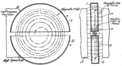 in which the particle moves in a planar spiral in a perpendicular magnetic field, given an electric kick every half turn, the increase in speed increases orbit size, but (nonrelativistically) the orbit time is constant, so an AC field can be used to provide the acceleration. The particles can be fed in continuously near the center of the machine, and spiral out to the maximum radius.  However, to increase speed into the relativistic range, the increase in mass means that the orbital time is no longer independent of energy.  Some lagging can be tolerated, but obviously not much.

Therefore, the particles must be fed into the machine one bunch at a time (rather than continuously) and the timing of electrical impulses then synchronized with the orbital time for the one bunch present, increasing with energy.  This is the synchrotron. The limiting factor for increasing energy in a synchrotron is that the particles circling are of course accelerating towards the center and therefore radiating energy.

Perhaps the most important synchrotron radiation facility is the Advanced Photon Source (APS) at Argonne National Lab. 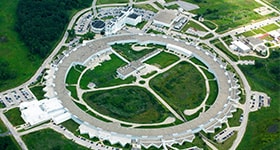 There electrons are accelerated to 7 Gev ( $\gamma \simeq 14,000$ ) and then sent into storage rings (1 km diameter) where rf fields are used to maintain their energy.  X-rays from this machine have recently made major contributions to finding the structure of important proteins, for example.

Summarizing Radiation Formulas

To analyze synchrotron radiation, we'll first summarize here the radiation formulas found so far.

First, the radiated power:

The nonrelativistic Larmor formula:

$$P=\frac{1}{6\pi {\epsilon }_0}\cdot \frac{a^2{q}^2}{c^3}=\frac{{\mu }_0}{6\pi }\cdot \frac{a^2{q}^2}{c},$$  and the relativistic generalization: $$P=\frac{{\mu }_{0}c{q}^2{\gamma }^6}{6\pi }{\left[{\dot{\beta }}^2-{\left(\beta \times \dot{\beta }\right)}^2\right]}_{\text{ret}}.$$  In linear motion, the second term of course disappears.

In circular motion at radius $r:$ 

$$P=\frac{{\mu }_0}{6\pi }\cdot \frac{q^2{c}^3}{r^2}{\beta }^4{\gamma }^4.$$  To find the pattern of radiation needs significantly more work.  We need the Lienard-Weichert formula for the electric field, the magnetic field radiated has essentially the same form, so we can find the Poynting vector in any direction.

 The electric field is: $$\overrightarrow{E}=\frac{q}{4\pi {\epsilon }_0{R}^2}{\left[\frac{\widehat{\overrightarrow{n}}-\overrightarrow{\beta }}{{\gamma }^2{\left(1-\overrightarrow{\beta }\cdot \widehat{\overrightarrow{n}}\right)}^3}\right]}_{\text{ret}}+\frac{q}{4\pi {\epsilon }_{0}cR}{\left[\frac{\widehat{\overrightarrow{n}}\times \left[\left(\widehat{\overrightarrow{n}}-\overrightarrow{\beta }\right)\times \dot{\overrightarrow{\beta }}\right]}{{\left(1-\overrightarrow{\beta }\cdot \widehat{\overrightarrow{n}}\right)}^3}\right]}_{\text{ret}}.$$  The first term is just the relativistic static field from the moving charge, the same as for a nonaccelerating (but moving) charge.  The second term is the radiation.

Circular Acceleration: Angular Distribution

Following Jackson, we take $\overrightarrow{\beta }=\beta \widehat{z},\dot{\overrightarrow{\beta }}=\dot{\beta }\widehat{x},\widehat{n}=\sin \theta \cos \varphi \widehat{x}+\sin \theta \sin \varphi \widehat{y}+\cos \theta \widehat{z}$ in $$\frac{dP\left(t_{\text{ret}}\right)}{d\Omega }={\left.\frac{{\mu }_{0}c{q}^2}{16{\pi }^2}\frac{{\left|\widehat{\overrightarrow{n}}\times \left[\left(\widehat{\overrightarrow{n}}-\overrightarrow{\beta }\right)\times \dot{\overrightarrow{\beta }}\right]\right|}^2}{{\left(1-\overrightarrow{\beta }\cdot \widehat{\overrightarrow{n}}\right)}^5}\right|}_{\text{ret}}.$$  to find with lots of algebra $$\frac{dP\left(t_{\text{ret}}\right)}{d\Omega }={\left.\frac{{\mu }_0{q}^2{\dot{v}}^2}{16{\pi }^{2}c}\cdot \frac{1}{{\left(1-\beta \cos \theta \right)}^3}\cdot \left[1-\frac{{\sin }^2\theta {\cos }^2\varphi }{{\gamma }^2{\left(1-\beta \cos \theta \right)}^2}\right]\right|}_{\text{ret}}.$$  Recall now $\beta$ is very close to one, $1-\beta \sim {10}^{-8},$ so this beam is well focused in the $\theta$ direction. Huge power per unit solid angle, but over a very small solid angle.

The Heaviside-Feynman Formula

The expression for the electric field of a moving point charge given above can be written in a quite different, rather simple, way (the derivation is nontrivial, sketched in Zangwill, detailed in Garg) first found by Heaviside, discovered independently by Feynman (and mentioned in his lectures):

$$\overrightarrow{E}\left(\overrightarrow{r},t\right)=\frac{q}{4\pi {\epsilon }_0}\left\{{\left[\frac{\widehat{n}}{R^2}\right]}_{\text{ret}}+\frac{R_{\text{ret}}}{c}\frac{d}{dt}{\left[\frac{\widehat{n}}{R^2}\right]}_{\text{ret}}+\frac{1}{c^2}\frac{d^2{\widehat{n}}_{\text{ret}}}{d{t}^2}\right\},$$ 

and the magnetic field is given by

$$c\overrightarrow{B}\left(\overrightarrow{r},t\right)={\widehat{n}}_{\text{ret}}\times \overrightarrow{E}\left(\overrightarrow{r},t\right).$$ 

This is an appealing formulation, because the terms can be made plausible intuitively:

The first term is the ordinary Coulomb field from the retarded time (position).

The second term more or less updates the field to the one we are now familiar with, the "squashed" Coulomb field for a charge moving at constant velocity, centered at the actual (current) position of the charge.

  The third term includes the radiative field from the charge's acceleration, notice it's the acceleration in the observer's time of the unit vector pointing from the observer to the retarded particle position. (Some treatments take the reverse of this vector$—$it doesn’t matter).  We can see that this is a radiation field because the acceleration of a unit vector tracking motion at a distance $R$ will be attenuated by a factor $1/R.$ Furthermore (see Purcell’s picture given here) the accelerated charge  radiates most intensely  in the equatorial plane, and using the unit vector automatically picks this transverse acceleration.  

The above discussion of the terms is handwaving, but since the complete formula is in fact exact, approximations in our interpretation must cancel!

Synchrotron Radiation

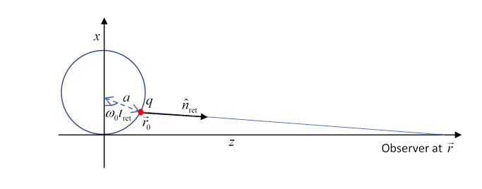
The circle represents the synchrotron, radius $a,$ and a charge $q$ at angle ${\omega }_0{t}_{\text{ret}}.$ The observer is taken to be very far away in the $z$ direction.  The unit vector ${\widehat{n}}_{\text{ret}}$ points to the observer from the apparent position of the charge, that is, where it was at the retarded time$—$in other words, where the observer sees it to be.

$${\overrightarrow{r}}_0\left(t_{\text{ret}}\right)=a\left(1-\cos {\omega }_0{t}_{\text{ret}}\right)\widehat{x}+a\sin \left({\omega }_0{t}_{\text{ret}}\right)\widehat{z}.$$  Now the vector ${\widehat{n}}_{\text{ret}}=\left[\overrightarrow{r}-{\overrightarrow{r}}_0\left(t_{\text{ret}}\right)\right]/R_{\text{ret}}$ where $\overrightarrow{R}=\overrightarrow{r}-{\overrightarrow{r}}_0,$ and to a good approximation $R_{\text{ret}}=r-a\sin \left({\omega }_0{t}_{\text{ret}}\right),$ so

$${\widehat{n}}_{\text{ret}}=\frac{a\left(\cos {\omega }_0{t}_{\text{ret}}-1\right)\widehat{x}+\left[r-a\sin \left({\omega }_0{t}_{\text{ret}}\right)\right]\widehat{z}}{r-a\sin \left({\omega }_0{t}_{\text{ret}}\right)}.$$ Notice now the $\widehat{z}$ component is time-independent, and in the $\widehat{x}$ component we can just keep the $r$ in the denominator, so Feynman's formula for the radiating electric field becomes

$$\overrightarrow{E}\left(\overrightarrow{r},t\right)=\frac{q}{4\pi {\epsilon }_0{c}^2}\frac{d^2{\widehat{n}}_{\text{ret}}}{d{t}^2}=\frac{q\widehat{x}}{4\pi {\epsilon }_0{c}^2}\frac{d^2}{d{t}^2}\frac{a\cos {\omega }_0{t}_{\text{ret}}}{r}.$$Now

$$c\left(t-t_{\text{ret}}\right)=r-a\sin \left({\omega }_0{t}_{\text{ret}}\right),$$Rearranging, and using $\beta c=a{\omega }_0,$ and incorporating the constant $r/c$ into the observer's clock setting,

$${\omega }_{0}t={\omega }_0{t}_{\text{ret}}-\beta \sin \left({\omega }_0{t}_{\text{ret}}\right).$$ Again use $\beta c=a{\omega }_0$ to write

$$\overrightarrow{E}\left(\overrightarrow{r},t\right)=\frac{q\widehat{x}}{4\pi {\epsilon }_{0}c{\omega }_0}\frac{d^2}{d{t}^2}\frac{\beta \cos {\omega }_0{t}_{\text{ret}}}{r}.$$  These two equations describe a curve parameterized by $t_{\text{ret}}.$ We need to plot $\beta \cos {\omega }_0{t}_{\text{ret}}$ against ${\omega }_{0}t$ and find its second derivative to find $\overrightarrow{E}\left(\overrightarrow{r},t\right)$ as a function of observer time $t.$ 

In fact, this is a generalized cycloid: imagine rolling a wheel of unit radius along a horizontal line, and track a point on the wheel a distance $\beta$ from the center.  Now $t_{\text{ret}}$ is how long the wheel has been rolling, with angular velocity ${\omega }_0.$  Its center will have moved through ${\omega }_0{t}_{\text{ret}}$ horizontally, the point is horizontally $-\beta \sin \left({\omega }_0{t}_{\text{ret}}\right)$ from the center, and vertically displaced by  $\beta \cos \left({\omega }_0{t}_{\text{ret}}\right).$ 

If the spot is at the center of the wheel, $\beta =0,$ the radiated field is zero.  If $\beta \ll 1,$ the electric field oscillates sinusoidally with frequency ${\omega }_0.$  But as $\beta \to 1,$ the curve approaches an actual cycloid, tending to a cusp, the second derivative goes to infinity.  The radiation becomes a series of pulses.

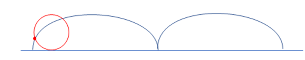
To get a clear picture of just how the curve goes from a sinusoidal oscillation in the low speed limit to approaching a cycloid in the extreme relativistic limit, click here. The high energy limit corresponds to unit radius (the default setting, easily adjusted). By the way, the cycloid picture in Zangwill (page 895) is incorrect: the intermediate curve should of course be smooth, the cusp only comes in the relativistic limit.

Note on this cycloid curve:  the standard notation would be $x=\theta -\beta \sin \theta ,y=1-\beta \cos \theta ,$ with almost cusp at $\theta =0$ for $\beta \to 1.$  Near the origin,  $x\cong \left(1-\beta \right)\theta ,y\cong 1-\beta +\frac{1}{2}{\theta }^2$ so $d^{2}y/d{x}^2\cong 1/{\left(1-\beta \right)}^2.$  

This tells us the curvature at the cusp compared with the curvature of the rest of the curve (of order unity) is up by a factor of ${\gamma }^4.$ 

The Advanced Photon Source has radius one kilometer, so the circling frequency is of order 100 kHz.  At that frequency, the wavelength radiated would be of order a kilometer.  But near the cusp this is shortened by a factor of order ${\gamma }^4,$ and $\gamma \sim {10}^4,$ and the radiation is X-rays. 

Cosmic Synchrotron Radiation

Synchrotron radiation is common in astronomy. Of course, it signals the presence of magnetic fields, so gives extra insight into the systems being studied. It has helped understand Jupiter's magnetosphere. It is present in the remnants of supernovae, electrons in a magnetic field give fairly well polarized bright radiation, but also are transparent.  Synchrotron radiation from neutron stars suggests magnetic fields of order 10⁸ tesla. 

previous  index  next