previous  index  next 

73.  Motion of a Charge e in Static Electric and/or Magnetic Field(s)

Michael Fowler, UVa

Jackson 12.2, 12.3

Constant Electric Field

The equation of motion is

$$\frac{d\overrightarrow{p}}{dt}=e\overrightarrow{E},\overrightarrow{p}=\gamma m\overrightarrow{v},\gamma =1/\sqrt{1-\left(v^2/c^2\right)}.$$

For nonrelativistic motion $\gamma =1$ and the path is the same as an object in a uniform gravitational field, that is, the motion is parabolic. 

The relativistic case is given as a problem in Jackson (12.3), here we’ll review Landau’s presentation (Landau page 55).

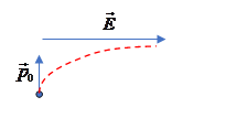
Take the constant electric field to be in the $x$ -direction, the initial momentum to be $p_0$ in the $y$ -direction. The dotted curve suggests a path.

The equations of motion ${\dot{p}}_x=eE,{\dot{p}}_y=0$ integrate with obvious boundary conditions to

$$p_x=eEt,p_y=p_0.$$

Notation:  In this section, we’re following Landau’s use of $\mathcal{E}$ for energy, keeping $E$ for the electric field.

The kinetic energy of the particle (following Landau’s definition, so including rest mass) is given by

$${\mathcal{E}}_{\text{kin}}^2=m^2{c}^4+c^2{p}^2.$$

We’ll write ${\mathcal{E}}_{\text{kin}}^2\left(t=0\right)=m^2{c}^4+c^2{p}_0^2={\mathcal{E}}_0.$ 

 With Landau’s definition, then,  ${\mathcal{E}}_{\text{kin}}=\gamma m{c}^2,\overrightarrow{p}=\gamma m\overrightarrow{v}=\left({\mathcal{E}}_{\text{kin}}/c^2\right)\overrightarrow{v}.$ 

Then

$${\mathcal{E}}_{\text{kin}}=\sqrt{m^2{c}^4+c^2{p}_0^2+{\left(ceEt\right)}^2}=\sqrt{{\mathcal{E}}_0^2+{\left(ceEt\right)}^2},$$

 and

$$\frac{dx}{dt}=\frac{p_x{c}^2}{{\mathcal{E}}_{\text{kin}}}=\frac{c^{2}eEt}{\sqrt{{\mathcal{E}}_0^2+{\left(ceEt\right)}^2}}.$$

This easily integrates to

$$x=\frac{1}{eE}\sqrt{{\mathcal{E}}_0^2+{\left(ceEt\right)}^2}.$$

The special case $p_0=0$ corresponds to constant acceleration in the moving object’s frame, since the horizontal electric field is not changed by going to another frame with horizontal relative motion.

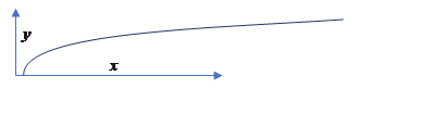
To find the path shape for $p_0\ne 0,$

$$\frac{dy}{dt}=\frac{p_y{c}^2}{{\mathcal{E}}_{\text{kin}}}=\frac{p_0{c}^2}{\sqrt{{\mathcal{E}}_0^2+{\left(ceEt\right)}^2}},$$

integrating to

$$y=\frac{p_{0}c}{eE}{\sinh }^{-1}\left(\frac{ceEt}{{\mathcal{E}}_0}\right).$$

The charge therefore moves along the catenary curve

$$x=\frac{{\mathcal{E}}_0}{eE}\cosh \frac{eEy}{p_{0}c}.$$

Thinking of the catenary as the shape of a rope hanging between two pegs at the same height, our curve is (half of) that, and of course rotated by ninety degrees. 

Exercise: Check the nonrelativistic limit.

The acceleration of a charge to relativistic speeds corresponds to a rope much longer than the distance between the pegs, the bottom point of the rope corresponds to the initial position.   

Note that since the momentum in the $y$-direction is constant, the velocity in that direction goes down as the charge reaches relativistic speeds, and distance from the $x$-axis increases with time very slowly indeed. (Exercise: how slowly?)

Constant Magnetic Field: Larmor Radius

Jackson 12.2

 Here we’re following Jackson, using G units, so electric and magnetic fields have same dimension, hence velocity term must be $v/c,$ but we’ll use $\mathcal{E}$ for energy

$$\frac{d\overrightarrow{p}}{dt}=e\frac{\overrightarrow{v}}{c}\times \overrightarrow{B}=e\overrightarrow{\beta }\times \overrightarrow{B},\frac{d\mathcal{E}}{dt}=0$$

the magnetic force does no work (and we’re taking zero electric field here) so $\left|\overrightarrow{v}\right|$ and $\gamma$ remain constant. Hence

$$\frac{d\overrightarrow{v}}{dt}=\overrightarrow{v}\times {\overrightarrow{\omega }}_{\overrightarrow{B}},{\overrightarrow{\omega }}_{\overrightarrow{B}}=\frac{e\overrightarrow{B}}{\gamma mc}=\frac{ec\overrightarrow{B}}{\mathcal{E}}.$$

The path is circular motion in the plane perpendicular to the magnetic field, with angular frequency ${\omega }_{\overrightarrow{B}},$ plus uniform linear motion in the direction of the field, combining to helical motion, in obvious notation

$$\overrightarrow{x}\left(t\right)={\overrightarrow{X}}_0+v_{\parallel }t{\overrightarrow{\epsilon }}_3+ia\left({\overrightarrow{\epsilon }}_1-i{\overrightarrow{\epsilon }}_2\right)e^{-i{\omega }_{\overrightarrow{B}}t}.$$

Exercise: Check that the real part of this expression gives the path described.

The circular motion perpendicular to the field is sometimes termed a Larmor circle, with Larmor radius (Jackson calls it the gyration radius):

$$a=\frac{c{p}_{\perp }}{eB}.$$

 Here $p_{\perp }$ is the magnitude of the momentum component perpendicular to the magnetic field.

The circling charge is equivalent to a current $j=\left(e/2\pi a\right)\left(p_{\perp }/\gamma m\right),$ and hence an orbital magnetic moment                   $$\mu =\frac{\pi a^{2}j}{c}=\frac{ea{p}_{\perp }}{2\gamma mc}=\frac{c{p}_{\perp }^2}{2Bc}=\frac{e{\omega }_B{a}^2}{2c}.$$ Warning!  Remember we’re in Gaussian units at the moment, where magnetic moment of current loop is current $\times$ area $/c.$

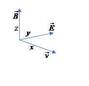
Constant Orthogonal Electric and Magnetic Fields

We’ll take constant fields $\overrightarrow{E}=\left(0,E_y,0\right),\overrightarrow{B}=\left(0,0,B_z\right).$

A charged particle moving at steady speed $v=c\beta$ along the $x$ -axis will feel a force (G units)

$$\overrightarrow{F}=e\left(\overrightarrow{E}+\overrightarrow{\beta }\times \overrightarrow{B}\right)=e\left(E_y-\beta B_z\right)\widehat{\overrightarrow{y}}$$

This force will be zero if (check this!)

$$\overrightarrow{\beta }=\frac{\overrightarrow{E}\times \overrightarrow{B}}{B^2}.$$

(This is of course the standard method for sorting particles by velocity$—$for a linear stream of particles of differing velocities, only those with this velocity will have electric and magnetic forces cancelling, and so be undeviated.)

Note also that this doesn’t depend on the sign of the charge, both treated the same.

To put this another way, for the given fields the particle moving at $\overrightarrow{v}$ does not accelerate, so therefore cannot be feeling an electric field in its own (rest) frame of reference. To see this explicitly, here are the fields in that frame (from lecture 64, for an $x$ -direction boost, also Jackson 11.148, now Gaussian):

$$\begin{array}{l}{E^{\prime }}_y=\gamma \left(E_y-\beta B_z\right),\\ {B^{\prime }}_z=\gamma \left(B_z-\beta E_y\right).\end{array}$$ 

(And also ${\overline{E}}_x=E_x,$ ${\overline{B}}_x=B_x.$ )

Hence if $v/c=\beta =E_y/B_z,$ the particle sees only a magnetic field, of strength

$${B^{\prime }}_z=\gamma \left(1-{\beta }^2\right)B_z=B_z/\gamma .$$

Therefore, the motion of the electron in the crossed electric and magnetic fields is just that of an electron in the (weaker) magnetic field (described above), plus the perpendicular drift velocity $cE/B.$

Obviously, though, the electron isn’t moving faster than light, so we have evidently assumed that $E<B$ (in gaussian units, of course: $E<cB$ in SI).

If for the static fields $E>B,$ at speed $v/c=B/E,$ in the moving frame there is only an electric field, giving the catenary curve plus the constant perpendicular drift velocity.

Note: As discussed in lecture 65, a purely electric field in one frame cannot transform to a purely magnetic field in another frame: $E^2-c^2{B}^2$ is a Lorentz invariant (as is $\overrightarrow{E}\cdot \overrightarrow{B},$ so if the fields are not perpendicular, there is no frame in which they are. )

Exercises: These are from Landau, where you can find the full solutions. (But try them first!)

1.   Determine the relativistic motion of a charge in parallel uniform electric and magnetic fields.

Hint: First find the motion along the common field direction, then prove that the magnitude of the momentum component in the perpendicular plane is constant. A parametric answer is fine.

2.      Determine the relativistic motion of a charge in perpendicular electric and magnetic fields of equal magnitude.

Hint: Taking $\overrightarrow{E}=\left(0,E_y,0\right),\overrightarrow{B}=\left(0,0,B_z\right),$ show that $p_z$ is constant, and ${\mathcal{E}}_{\text{kin}}-c{p}_x=\alpha$ is constant. Then find ${\mathcal{E}}_{\text{kin}},p_x,t$ as functions of $p_y.$ This parameterizes the path.  An equivalent approach is outlined in Jackson problem 12.6.

previous  index  next