74  Particle Drift in Nonuniform Static Magnetic Field: Guiding Center Motion

Michael Fowler  UVa

Jackson 12.4

Guiding Center

We’ve found that in a uniform magnetic field a particle moves in a path that is a combination of circling around a field line (in a circle with radius proportional to the speed of the particle) and a steady speed of the center of the circle$—$the guiding center$—$in the direction of the field.

We’ll now consider a slowly spatially varying (static) magnetic field: in particular, one that varies little over the radius of the particle’s circular motion.  (So we’re also restricting the energy range of the particle.)  The first approximation to the motion is still that of spiraling around a field line, but that neglects other important effects.

 Here we’ll examine two kinds of field variation that give rise to guiding center drift perpendicular to the local field direction, that is, sideways:

 1.   A gradient in field magnitude, and

 2.   Curvature of field lines.

Particle Moving in (x,y) Plane, Varying Strength z-Direction Field: Gradient Drift

We’ll begin with a very crude example to illustrate the essential physics, and for simplicity take the nonrelativistic limit.

Suppose the magnetic field points in the $z$-direction, and is almost constant, but is linearly increasing in magnitude in the $x$-direction.  To simplify even further, we  suppose the field has magnitude $B_1$ for $x<0$ and $B_2=B_1+\Delta B$ for $x>0:$ just replacing the linear increase with a simple small step.

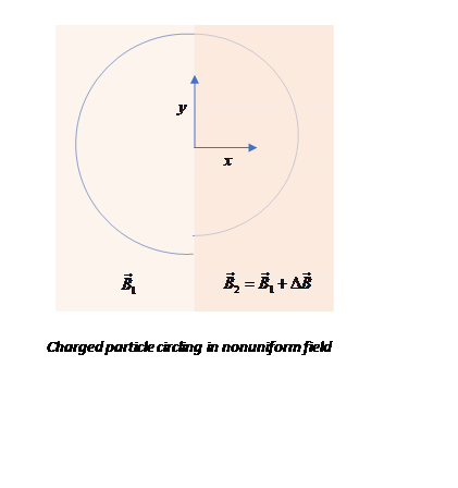
Now consider a charged particle circling in the field in the $x,y$ plane.  Suppose we start at the bottom point of the curve shown in the diagram, on the $y$-axis, the particle moving in the negative $x$-direction at speed $v_{\perp }$ (which stays constant throughout). Moving in the weaker field ${\overrightarrow{B}}_1,$ the particle traces a half-circle of radius $r_1,$ where

$$v_{\perp }={\omega }_{B_1}{r}_1,{\omega }_{B_1}=\frac{e{B}_1}{mc}.$$

The particle crosses into the incrementally stronger field at a point $2r_1$ above the original entry point. After a downward half-circle in the stronger field, the particle is close to the original entry point, but vertically displaced by an amount

$$\Delta y=2\left(r_1-r_2\right)=2v_{\perp }\left(\frac{1}{{\omega }_{B_1}}-\frac{1}{{\omega }_{B_2}}\right)\approx 2v_{\perp }\frac{\Delta {\omega }_B}{{\omega }_B^2}\approx \frac{2v_{\perp }mc}{e}\frac{\Delta B}{B^2}.$$

The particle’s velocity at this point is identical in magnitude and direction to its initial value, so the path will repeat, just displaced vertically.  That is, after $\Delta t=2\pi /{\omega }_B$ the model predicts that the orbit will have moved in the $y$-direction by $\Delta y$ given above, and writing $v_{\perp }=\omega r$ and $mc/eB=1/\omega ,$ we find to first order the obvious result

$$\Delta y\approx 2r\Delta B/B$$

and therefore a net drift velocity perpendicular to the field

$$v_{\text{G model}}=\frac{\Delta y}{\Delta t}=\frac{2r\Delta B/B}{2\pi /\omega }=r\omega \frac{\Delta B}{B}.$$

The crude part of our model is just taking two possible magnetic field values, to represent a smoothly varying field. To compare our result with Jackson’s more precise analysis we write

$$\Delta B\approx r\nabla B,$$

to give

$$v_{\text{G model}}\approx r^2{\omega }_B\nabla B/B\approx \left(v_{\perp }^2/{\omega }_B\right)\nabla B/B.$$

Comparing this naïve result with Jackson’s 12.55, $v_G=\left(\omega r^2/2B^2\right)\left(\overrightarrow{B}\times {\nabla }_{\perp }B\right),$ we see that the simple model automatically gives the direction of the drift velocity (see diagram) as perpendicular to the magnetic field and to the direction of its gradient. However, the magnitude is off by a factor of 2: the proper way to find the net vertical displacement is to integrate around the orbit using the linearly varying magnetic field.  It’s fairly straightforward, see Jackson for details, the corrected result is:

$$v_{\text{G}}=\left(v_{\perp }^2/2{\omega }_B\right)\nabla B/B.$$

Notice that the direction of the drift is also perpendicular to the gradient (hence subscript G) of the magnetic field strength. This means the particle will drift along an “equipotential” of magnetic field strength. Suppose now the magnetic field strength is zero beyond a certain distance $R$ from the origin. Then the “equipotentials” must be closed curves, and an electron moving within this region will never get out!  Of course, it has to be moving slowly enough for our approximations to be valid.  This problem has been fully discussed by a famous physicist: Edward Witten, Annals of Physics 120, 72 (1979).

Drift Velocity from Field Lines Curvature

Obviously, the field lines in general curve, taking them straight in the example above was an approximation. To see what difference arises from curved field lines,  Jackson (page 591) takes as an example field lines from a line of current along the $z$-axis, that is, circles in the $\left(x,y\right)$ plane, the same irrotational vector field as the fluid velocity field around a whirlpool.

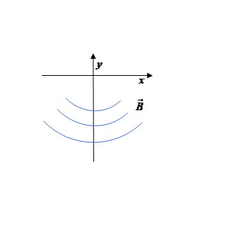
Now assume with Jackson that the particle is tightly spiraling around a field line which is an arc of a circle of radius $R,$ with net velocity $v_{\parallel }$ along the field line.  This net motion has acceleration $v_{\parallel }^2/R$ towards the $z$-axis,  equivalent to motion in an effective radial electric field $E_{\text{eff}}=\left(m/eR\right)v_{\parallel }^2.$ Recalling that crossed electric and magnetic fields give a drift velocity $c\overrightarrow{E}\times \overrightarrow{B}/B^2,$ we find the drift velocity from this field curvature $v_C$ to be (using ${\omega }_B=eB/mc$ ) in the $z$-direction, with magnitude

$$v_C=v_{\parallel }^2/{\omega }_{B}R.$$

For the effectively two-dimensional magnetic field we are considering, $\overrightarrow{\nabla }\times \overrightarrow{B}=0$ means ${\nabla }_{\perp }B/B=-\overrightarrow{R}/R^2,$ and recalling from the previous section that the drift velocity from a field gradient is $v_{\text{G}}=\left(v_{\perp }^2/2{\omega }_B\right)\nabla B/B,$ evidently in the $z$-direction here (since $\overrightarrow{B}$ is azimuthal and $\overrightarrow{\nabla }B$ is radial), the two drift velocities can be added, yielding total

$$v_{\text{drift}}=\left(1/{\omega }_{B}R\right)\left(v_{\parallel }^2+\frac{1}{2}{v}_{\perp }^2\right).$$

Note that the drift depends on the sign of the charge through ${\omega }_B$ so in a plasma charges would separate, in contrast to movement induced by crossed electric and magnetic fields.

Containing Hot Plasma

These drifts are problematic in machines designed to contain a hot plasma, such as attempts at nuclear fusion, where ions are typically inside some kind of toroid. Billions of dollars have been spent designing magnetic containment chambers, but so far none have been successful in holding significant nuclear fusion. For an interesting attempt, click stellarator.

Earth’s Ring Current

As we’ll discuss later, this sideways drift acts on the particles in the van Allen radiation belts to generate a ring current around the Earth, which is enough, during magnetic storms, to partially cancel the Earth’s magnetic field, and thus allow more cosmic radiation to reach the Earth’s surface.

previous  index  next