previous  index  next 

75  Adiabatic Invariants for a Charged Particle Moving in a Slowly Varying Magnetic Field

Michael Fowler  UVa

Jackson 12.5

Guiding Center Picture

As we’ve seen in the previous lectures, it turns out that, over a wide range of particle energies and field strengths, the motion of a charged particle in a slowly varying magnetic field is well-described as moving in tight small circles (sometimes called Larmor circles) around a guiding center, which itself moves slowly.  And, by “slowly” we mean the guiding center moves only a small fraction of the small circle radius during each revolution, so the particle’s path is almost closed, the motion almost repeats. For a constant magnetic field, the guiding center moves along the field direction. We showed in the last lecture that the guiding center will also drift sideways if the field strength varies or if the field lines are curved.

 In this lecture, we’ll consider the center moving along a field line with negligible curvature, but moving into a region where the field strength is changing significantly. This is different from the previous cases:  here the size of the Larmor circle can change in an essential way. 

Adiabatic Invariants:  A Clue from the Old Quantum Theory

To think about how the Larmor circle itself might change on drifting into a region of different magnetic field strength, it’s instructive to consider a bit of ancient quantum history, where we’ll find a very similar situation.  The first semi-successful model of an atom was Bohr’s hydrogen model, with electrons in circular orbits around the proton, but arbitrarily (it seemed) restricted in angular momentum$—$which could only be $nh/2\pi ,$ with $n$ an integer and  $h$ Planck’s constant (already known at the time from black body radiation). This recipe led to all the energy levels spectroscopically observed$—$a fantastic triumph.

But still, what was the justification? Why these radii, and what about elliptical orbits?  After all, the force was inverse square$—$just like gravity, which certainly has elliptic orbits.

A rationale for the allowed radii was first suggested by  de Broglie, who conjectured that the electron had a wavelike nature, with wavelength depending on momentum using the same formula already familiar for photons, $p=h/\lambda .$  The allowed circular orbits were then those that contained a whole number of wavelengths $\lambda :$ so the wave fit smoothly and uninterrupted around the path. This idea worked!

It’s often shown in textbooks as a real standing wave fitting around the circle, but here we’ll take the angular momentum eigenstates, traveling wavefunctions, proportional to $e^{ipx/\hslash }$ with $x$ measuring distance along the path. In the n^th state, this complex-valued wave function $\psi \left(x\right)$ circles the complex $\psi$ plane origin n times as $x$ goes once around the real space path. ( The real, standing wave representation usually shown just takes the sum and difference of these traveling wave angular momentum eigenstates.)

But wait, what about the elliptical orbits?  Why can we ignore them? Sommerfeld solved that mystery by computing the general elliptical orbit, that is, solving to find the momentum variable $p(x)$ at all points $x$ along the orbit, and then requiring a whole number of$—$now variable$—$wavelengths to fit smoothly around the orbit,

$$\left(1/\hslash \right){\displaystyle ∳p\left(x\right)dx=2\pi n}.$$

Remarkably, this gives the identical same set of energies as the simple Bohr circular orbits!  So, they were there all along. This energy degeneracy for different shaped orbits is unique to the inverse square force$—$we got lucky, or rather Bohr did.

Picture now in this semiclassical spirit the general elliptical orbit in space, and the traveling complex wavefunction $\psi \left(x\right)$ around this orbit.   As $x$ goes one time around the orbit in ordinary space, the wavefunction $\psi \left(x\right)$ is a point circling the origin in its complex $\psi$ plane, completing exactly n turns, because as $x$ returns to the orbital starting point, $\psi \left(x\right)$ must go to the original position and slope, it must be a smooth wave function all the way around. 

But now suppose we add in some small slow change to the potential, perhaps another atom moves slowly into the neighborhood. This is termed an “adiabatic” change.  What happens to the wavefunction $\psi \left(x\right)$? Obviously, it will change. But, visualizing $\psi \left(x\right)$ circling around the origin in the complex $\psi$ plane as $x$ traces the physical path, unless the perturbing potential is strong enough to drive the wavefunction to zero at some point, the total number n of turns about the $\psi$ origin for the complete path will not change.

Note:  From a quantum perspective, the photon energy necessary for $\psi \left(x\right)$ to move up from n to n+1 turns is close to $h\nu ,$ with $\nu$ the inverse orbital time, so if external changes are small on a time scale set by the orbital time, the quantum number is very unlikely to change.

That is, for a particle in a periodic orbit, ${\displaystyle ∳p\left(x\right)dx}$ does not change when parameters such as the external field vary slowly. This is called an adiabatic invariant, adiabatic here meaning slow, smooth change.

 In classical mechanics, this adiabatic invariant is the action integral defined as

$$J=\left(1/2\pi \right){\displaystyle \oint pdq}$$

around one cycle, $q$ being an angle parameter and $p$ the canonical momentum.  This is fully discussed in my lecture.

History:  The connection to quantum mechanics was elucidated by Einstein and Sommerfeld at the Solvay Conference in 1911: in fact, the main conference agenda was attempting to reconcile classical and quantum physics.

The adiabatic invariant is the key to understanding how the Larmor orbit develops under smooth changes as it moves through the varying magnetic field.

Adiabatic Invariance of Flux Through Orbit of Particle

Magnetic Field and Wave Function Phase

We’ll consider field strengths, and particle momenta, to be such that the path is well-described (as in the preceding lecture) by a circling motion about a slowly moving guiding center, successive circles having centers much closer together than the circle radius.

We will continue in the semiclassical picture described above, and if we ignore the magnetic field, we would take the local wave function at a point on the ring $\sim e^{ipx/\hslash },$ with local kinetic momentum $p=\gamma mv,$ and going around the ring would yield a net phase increase of $2n\pi .$ (?)

But this is wrong! Recall (from lecture 72)  that to get the experimentally observed behavior of the classical electron in magnetic and electric fields we needed to add a term to the Lagrangian (in fact the simplest possible Lorentz invariant term linking the field to the particle)

$$S={\displaystyle \underset{a}{\overset{b}{\int }}Ldt}={\displaystyle \underset{a}{\overset{b}{\int }}\left(-m{c}^{2}d\tau -\frac{e}{c}{A}_{\mu }d{x}^{\mu }\right).}$$ so we see that adding the above term to the action is adding $eA/\hslash c$ to the phase of $\psi .$  With this addition, the waves correspond in wavelength to the canonical momentum

$$P_i=\frac{\partial L}{\partial u_i}=\gamma m{u}_i+\frac{e}{c}{A}_i.$$  

In other words, we’ve given a hand-waving semiclassical derivation for the adiabatic invariance of the classical action integral (with the canonical momentum!)

$$J={\displaystyle \oint P_{i}d{q}_i}.$$

Action Integral for Larmor Loop

The action corresponding to the circling motion ${\overrightarrow{v}}_{\perp }$ perpendicular to the field is

$$J={\displaystyle \oint {\overrightarrow{P}}_{\perp }\cdot d\overrightarrow{\ell }}={\displaystyle \oint \gamma m{\overrightarrow{v}}_{\perp }\cdot d\overrightarrow{\ell }}+\frac{e}{c}{\displaystyle \oint \overrightarrow{A}\cdot d\overrightarrow{\ell }}$$  In the adiabatic limit, we can take ${\overrightarrow{v}}_{\perp }\parallel d\overrightarrow{\ell }$ so  (with circle radius $a,v_{\perp }=a{\omega }_B,d\ell =ad\theta ,$ ${\omega }_B$ the circling frequency in field $B.$ )

$$\begin{array}{c}J={\displaystyle \oint \gamma m{\omega }_B{a}^{2}d\theta }+\frac{e}{c}{\displaystyle \oint \overrightarrow{A}\cdot d\overrightarrow{\ell },}\\ =2\pi \gamma m{\omega }_B{a}^2+\frac{e}{c}{\displaystyle \underset{S}{\int }\overrightarrow{B}\cdot \widehat{\overrightarrow{n}}da.}\end{array}$$  At this point, it's crucial to get the signs right, because these terms partially cancel.

Let's suppose the magnetic field is pointing in the positive $z$-direction, and the circling motion is therefore in the $x,y$ plane.  Take the particle to be positively charged, and think of the moment it crosses the positive $x$-axis, as it circles the origin. The force $(e/c)\overrightarrow{v}\times \overrightarrow{B}$ has to be towards the center of its circle, the origin, so it must be moving downwards, meaning circling clockwise.  Since it's part of the same integral, the ${\displaystyle \oint \overrightarrow{A}\cdot d\overrightarrow{\ell }}$ must also be taken clockwise, so that second integral must give

$$\frac{e}{c}{\displaystyle \underset{S}{\int }\overrightarrow{B}\cdot \widehat{\overrightarrow{n}}da}=-\frac{e}{c}\pi a^{2}B.$$  Noting that ${\omega }_B=eB/\gamma mc,$ we find the first term in $J$ is twice the magnitude of the second, and positive, so                                                                                     $$J=\frac{e}{c}\left(B\pi a^2\right).$$  This means that as the guiding center moves from a weak field to a strong field, the circle orbit will shrink to keep the same total magnetic flux through the circle.

Equivalent invariants are $p_{\perp }^2/B$ and $\gamma \mu ,$ where $\mu =e{\omega }_B{a}^2/2$ is the magnetic moment of the current loop.  (Exercise:  prove these!) 

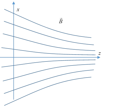
This invariant gives some insight into why a circling charged particle can be repelled by a magnetic pole, such as one of the Earth's magnetic poles. Jackson considers the case of a field mainly in the $z$-direction, but of varying strength:

 Imagine a charged particle, circling in the $x,y$ plane with velocity ${\overrightarrow{v}}_{\perp },$ but also coming in from the left with a nonzero drift velocity $v_{\parallel }$ in the $z$ -direction.

Since the only force on the particle is from the static magnetic field, its kinetic energy cannot change, $v_{\perp }^2+v_{\parallel }^2=v_0^2.$ 

From the adiabatic theorem, $$\frac{v_{\perp }^2}{B}=\frac{v_{\perp 0}^2}{B_0},$$ so $$v_{\parallel }^2=v_0^2-v_{\perp 0}^2\frac{B\left(z\right)}{B_0}.$$  This implies that motion in the $z$-direction is the same as a particle in a one-dimensional potential, evidently with a turning point if the field strength gets sufficiently strong to make the right-hand side zero.

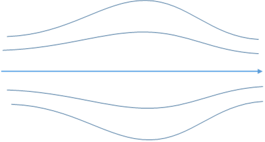
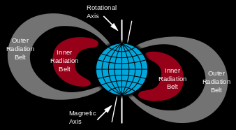
A charged particle can be confined in a "magnetic bottle" having field lines coming together at both ends.  This is the basic idea behind early attempts to confine a plasma at very high temperatures in hopes of gaining confined nuclear fusion.  Unfortunately, the one-particle model ignores sideways drift, and the plasma interactions occurring at finite density, which render the confinement unstable.

However, there are excellent examples in nature of this kind of magnetic bottle, such as the van Allen radiation belts, toroidally shaped region surrounding the Earth, and filled with charged particles.  These are shaped by the Earth's magnetic field (from Wikimedia Commons):