previous  index  next 

14. 2D Electrostatics: Complex Variable Methods I

    Michael Fowler, UVa

Introduction

If we have a function $w$ of a complex variable $z,$

$$w\left(x,y\right)=u\left(x,y\right)+iv\left(x,y\right),z=x+iy,u,v\text{ real,}$$

then in regions of the plane where $w\left(z\right)$ is differentiable, the real functions $u,v$ separately obey Laplace’s equation,

$${\nabla }^{2}u\left(x,y\right)=0,{\nabla }^{2}v\left(x,y\right)=0$$

and furthermore the two families of equipotentials intersect each other at right angles, so the equipotentials for potential $u\left(x,y\right)$ are the field lines for $v\left(x,y\right)$ and vice versa.

We’ll look at some simple examples.

Single Line of Charge

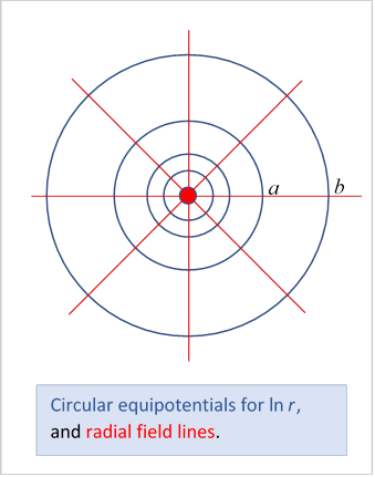
The potential from a single infinitely long line of charge of linear density $\lambda ,$ which we take along the $z$ -axis, is

$\phi \left(x,y\right)=\frac{\lambda }{2\pi {\epsilon }_0}\ln r,r=\sqrt{x^2+y^2}.$

From now on, we’ll drop the factor $\lambda /2\pi {\epsilon }_0$ and reinstate it at the end.

Now

$\ln z=\ln r{e}^{i\theta }=\ln r+i\theta$

is analytic (differentiable) everywhere except at the origin, so its real part,

$u\left(x,y\right)=\ln r,$

satisfies Laplace’s equation, and has as equipotentials circles centered at the origin.

Consider the annular space between the circles $r=a$ and $r=b.$ The potentials on these circles are $\ln a,\ln b$ respectively, the potential difference is $V=\ln \left(b/a\right).$

It follows from the uniqueness theorem that if we have a coaxial cable consisting of concentric cylindrical conductors, and the annular space between them has inner and outer radii $a,b,$ the field in that space must be as given here, for unit linear charge density, and hence the capacitance per unit length,

$$C=\frac{\lambda }{V}=\frac{2\pi {\epsilon }_0}{\ln \left(b/a\right)}.$$

An actual coaxial cable would have insulation plus probably dielectric, which we ignore$—$that can be adjusted for later.

Notice that in contrast to the three-dimensional case, where a single spherical conductor has a well-defined capacitance, a single cylinder does not. (Why? If you actually measured its capacitance by putting known charge on it and measuring the change in potential, what value, approximately, would you expect to find?)

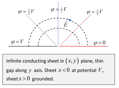
But what about the imaginary part of $\ln z$? That’s

$$\mathrm{Im}\ln z=v\left(x,y\right)=\theta .$$

This obeys ${\nabla }^{2}v=0,$ as you should check by finding the two-dimensional ${\nabla }^2$ in $\left(r,\theta \right)$ coordinates. But it’s not single valued:  if you go around once you add $2\pi .$ That doesn’t matter, of course, if the space is restricted so you can’t get all the way round.

The function $\phi =v\left(x,y\right)=\theta$ describes the potential in a region between two plates held at different potentials and meeting at an angle.  Looking at the single line diagram above , take the positive $x$-axis and the 45$˚$ line above it as the plates. The field lines are semicircles, the equipotentials are radial.

For another example, take both plates horizontal, as in this diagram:

Exercise:  Describe the charge distribution on the plates.

Wedges and Edges: Intersection of Grounded Plates

We’ll now examine the field in a region where two grounded flat conductors intersect, for example near an edge of a hollow grounded metal cube.  The potential is from faraway charges, plus the charge induced on the grounded plates. We’ll begin with the plates meeting at right angles.

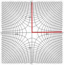
In the previous lecture, we discussed the real and imaginary parts of the analytic function $z^2.$  The imaginary part was $2xy,$ constant on a family of hyperbolae having the axes as asymptotes.  In particular, it was zero on the axes, the degenerate hyperbola.

This means these hyperbolae are the equipotentials for some field in a corner between two sheets of grounded conductor at right angles. 

The other hyperbolae are the field lines, going out perpendicular to the surface, as they must (parallel components would generate a current).

Focusing on the ++ quadrant, with the planes $x=0,y=0$ the grounded conductors, the picture above shows equipotentials and field lines near the corner for a charge far out along the 45$˚$ line.  In fact, we could have found it using images.

Exercise: Where and what are the appropriate image charges? 

What about two grounded sheets at 45$˚$ ? 

Clearly $\mathrm{Im}{z}^4$ will work for the equipotentials, $z^4$ having zero imaginary part on both sheets. (Write $z^4=r^4{e}^{4i\theta }.$ )  The equipotentials now are on curves of constant

$$\mathrm{Im}{z}^4=4xy\left(x+y\right)\left(x-y\right).$$

(Note where the zero equipotentials are.)  Again, this approximates the field near the corner from a faraway charge.

But $z^4$ is also a solution for the 90$˚$ case! How could that be?

Exercise:  For the 90$˚$ case, what about putting charges far out along the $\pi /8$ and $3\pi /8$ lines?   Would that give $z^4$ behavior near the corner? Do the charges have the same sign? Would images work? Do the grounded plates have induced charge with the same sign?

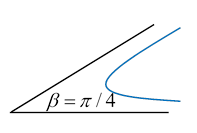
How about a general angle $\beta$ ?  Well, $z^{\pi /\beta }$ would work$—$so would $z^{m\pi /\beta },$ with $m$ an integer.  In general, the potential would be a series of such terms,

$\phi \left(\rho ,\varphi \right)=V+{\displaystyle \sum _{m=1}^{\infty }{a}_m{\rho }^{m\pi /\beta }\sin \left(m\pi \varphi /\beta \right)},$

dominated by the first close in to the corner (because it’s the lowest power) but needing the others to fit more distant boundary requirements.

The charge densities on the sides are given by the normal components of the electric fields, that is, the components in the $\varphi$ direction, taking only the leading term,

$$E_{\varphi }\left(\rho ,\varphi \right)=-\frac{1}{\rho }\frac{\partial \phi }{\partial \varphi }=-\frac{\pi a_1}{\beta }{\rho }^{\left(\pi /\beta \right)-1}\cos \left(\pi \varphi /\beta \right).$$

This will give the same sign charge density on both plates, that is, $-\frac{{\epsilon }_0\pi a_1}{\beta }{\rho }^{\left(\pi /\beta \right)-1}$.

Exercise: Will the image method work for any angle?

Opening Up

Notice from this expression that if $\beta =\pi$ the charge density is independent of $\rho$ near the corner$—$not surprising, because there isn’t a corner, we’ve flattened it! 

More interesting, if $\beta >\pi$ the charge density becomes infinite at the corner. 

Edge of a Conductor

The extreme case is $\beta =2\pi$, just a sharp edge of a conductor, where $\sigma \sim {\rho }^{-1/2}.$ So, if you have a charged infinitely thin conducting disc, for example, charge will pile up around the edge with this local density profile. There is still a finite amount of charge on integrating in from the edge, obviously.  We’ll return to this disc problem later: note the contrast with three dimensional objects, where all the charge on a conductor goes to the boundary.

Electrostatic Fields in Corners: Orthogonal Functions

We’ll momentarily take a break from the complex plane, and analyze ${\nabla }^2\phi =0$ in the usual cylindrical coordinate representation, following Jackson.

We’re dealing with ${\nabla }^2\phi =0$ in two dimensions, taking $\left(\rho ,\varphi \right)$ as the coordinates,

$$\frac{1}{\rho }\frac{\partial }{\partial \rho }\left(\rho \frac{\partial \phi }{\partial \rho }\right)+\frac{1}{{\rho }^2}\frac{{\partial }^2\phi }{\partial {\varphi }^2}=0$$

and take separable solutions

$\phi \left(\rho ,\varphi \right)=R\left(\rho \right)\Psi \left(\varphi \right)$

 to find

$$\frac{1}{R}\frac{d^{2}R\left(\rho \right)}{d{\rho }^2}={\nu }^2,\frac{1}{\Psi }\frac{d^2\Psi \left(\varphi \right)}{d{\varphi }^2}=-{\nu }^2,$$

having solutions

$R\left(\rho \right)=a{\rho }^{\nu }+b{\rho }^{-\nu },\Psi \left(\varphi \right)=A\cos \nu \varphi +B\sin \nu \varphi .$

How does these solutions translate to the complex number approach?  They’re just real and imaginary parts of simple powers, $z^{\nu },z^{-\nu }$!   (Remember $z^{\nu }=r^{\nu }{e}^{i\nu \theta }=r^{\nu }\left(\cos \nu \theta +i\sin \nu \theta \right)$.)  There is also, of course, a $\nu =0$ solution, just the log potential from a line of charge.

previous  index  next