previous  index  next 

15. 2D Electrostatics: Complex Variable Methods II

    Michael Fowler, UVa

Introduction

In the previous lecture, we focused on the functions $u\left(x,y\right),v\left(x,y\right)$ from the complex potential $\ln z,$ its real part the potential from a single line of charge, its imaginary part the potential between conducting plates at different potentials meeting along a line.

In this lecture, we’ll investigate the potentials from the complex expression for two parallel lines of charge. Remarkably, this provides straightforward solutions to some tough Jackson problems: 2.8, 2.13, 2.14, possibly others. And, in this approach the equipotentials are apparent from the start, whereas the infinite series solutions give almost no insight without a lot of further work.

Two Parallel Lines of Charge

We take two infinite line charges, linear charge density $\pm \lambda ,$ in the $z$-direction, located at $x=\pm a,y=0.$ 

Omitting the overall factor $\frac{\lambda }{2\pi {\epsilon }_0}$ to reduce clutter, the potential is the real part of the function

$$w\left(x,y\right)=u\left(x,y\right)+iv\left(x,y\right)=\ln \left(\frac{z-a}{z+a}\right),z=x+iy,a\text{ real}\text{.}$$

That is, the potential is:

$$u\left(x,y\right)=\mathrm{Re}\ln \left(\frac{z-a}{z+a}\right)=\ln \frac{\left|z-a\right|}{\left|z+a\right|}.$$

The equipotentials are therefore given by

$$\left|z-a\right|=e^u\left|z+a\right|.$$

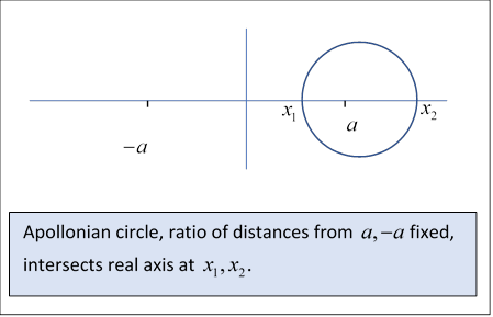
That is to say, the points in the plane at potential $u$ are those whose distances from the points $a,-a$ are in the same ratio $e^u.$ But we met this condition previously, in finding the image point for a charge outside a grounded sphere: these are the circles of Apollonius. (First found by the Greeks using geometric arguments, but you can easily verify the result with $\left(x,y\right)$ coordinates, and you can show the center is on the line through the two points, as it must of course be from symmetry.)

Our first task is to find the center and the radius of the circle corresponding to potential $u.$

Applying the above distance ratio formula to the points $x_1,x_2$ where the circle cuts the real axis,

$\begin{array}{l}{e}^u\left(a-x_1\right)=x_1+a,\\ e^u\left(x_2-a\right)=x_2+a.\end{array}$

Adding:

$e^u\left(x_2-x_1\right)=x_1+x_2+2a.$

Multiplying by $e^{-u}$ and subtracting,

$e^{-u}\left(x_2-x_1\right)=x_1+x_2-2a.$

Subtracting,

$$x_2-x_1=\frac{4a}{e^u-e^{-u}}=2a\mathrm{csch}u=2R,$$

where $R$ is the radius of the circle, and adding,

$$2\left(e^u+e^{-u}\right)R=2\left(x_1+x_2\right)=4d,$$

where $d$ is the distance of the circle center from the origin, so

$R=a\mathrm{csch}u,d=a\coth u.$

Capacitance of Two Parallel Circular Cylinders

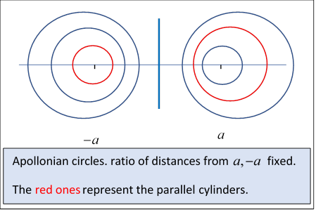
We’re now ready to consider the capacitance of two parallel circular cylinders using this result.

Recall

$\left|z-a\right|=e^u\left|z+a\right|.$

Evidently, from the diagram, the $y$-axis, equidistant from both lines of charge, is the curve for $u=0,$ and from the symmetry of the diagram, $-u$ and $u$ correspond to circles of the same radius the same distance from the $y$-axis in opposite directions.

We’ll take equipotentials at $u_1,u_2$ on opposite sides of the $y$-axis, having (from the end of the previous section) radii $R_{1,2}=a\left|\mathrm{csch}{u}_{1,2}\right|$ and centers separated by $D=a\left(\left|\coth u_1\right|+\left|\coth u_2\right|\right).$

The potential difference (which is what we need to evaluate the capacitance) is of course $\left|u_1-u_2\right|,$ but to evaluate this in terms of the radii and separation, which are all given in terms of hyperbolic functions of $u_1,u_2,$ obviously we must first find $\cosh \left(u_1-u_2\right)$ then invert it to get the answer.

Now

$$\begin{array}{c}\cosh \left(u_1-u_2\right)=\cosh u_1\cosh u_2-\sinh u_1\sinh u_2\\ =\frac{\coth u_1\coth u_2-1}{\mathrm{csch}{u}_1\mathrm{csch}{u}_2}.\end{array}$$

We have cylinder center separation squared (and using ${\coth }^2=1+{\mathrm{csch}}^2$ )

$$\begin{array}{c}{D}^2=a^2{\left(\left|\coth u_1\right|+\left|\coth u_2\right|\right)}^2\\ =R_1^2+a^2+R_2^2+a^2+2a^2\left|\coth u_1\right|\left|\coth u_2\right|\\ =R_1^2+R_2^2+2a^2\left(1-\coth u_1\coth u_2\right),\end{array}$$

In going to the last line, remember that $u_1,u_2$ have opposite signs, so

$$\cosh \left(u_1-u_2\right)=\frac{\coth u_1\coth u_2-1}{\mathrm{csch}{u}_1\mathrm{csch}{u}_2}=\frac{D^2-R_1^2-R_2^2}{2R_1{R}_2},$$

and the capacitance is (finally restoring the $2\pi {\epsilon }_0$ we removed at the beginning)

$$C=\frac{Q}{V}=\frac{2\pi {\epsilon }_0}{{\cosh }^{-1}\left(\frac{D^2-R_1^2-R_2^2}{2R_1{R}_2}\right)},$$

since we took unit linear charge density.

If one cylinder is inside the other, the same analysis carries through, except that the argument of the ${\cosh }^{=1}$ gains a minus sign.

Exercise: Check that for two parallel wires, radii $R,$ distance $d\gg R$ apart, $C\cong \pi \epsilon /2\ln \left(d/R\right).$

Note: In the literature, for two cables of diameter $d$ with centers $s$ apart, the capacitance is given as $C=\pi {\epsilon }_0/{\cosh }^{-1}\left(s/d\right).$ This is equivalent to our result: put

$$x={\cosh }^{-1}\left(\frac{D^2}{2R^2}-1\right)={\cosh }^{-1}\left(\frac{2s^2}{d^2}-1\right),$$

switching to the more common notation, so

$$\cosh x=\frac{2s^2}{d^2}-1=2{\cosh }^2\left(\frac{x}{2}\right)-1.$$

Hence $x=2{\cosh }^{-1}\left(s/d\right).$

Problems in Split Pipes

We’ve just found the potential from two parallel infinite line charges, $\pm \lambda ,$ in the $z$-direction, located at $x=\pm a,y=0,$ to be the real part of the function

$$w\left(x,y\right)=u\left(x,y\right)+iv\left(x,y\right)=\ln \left(\frac{z-a}{z+a}\right),z=x+iy,a\text{ real}\text{.}$$

But we know that the imaginary part also satisfies Laplace’s equation: ${\nabla }^{2}v\left(x,y\right)=0,$ except at the two singular points. What system of charges could that represent?

Writing

$$\begin{array}{l}z-a=r_1{e}^{i{\theta }_1},\\ z+a=r_2{e}^{i{\theta }_2},\end{array}$$

Evidently the potential is

$$v\left(x,y\right)={\theta }_1-{\theta }_2,$$

and equipotentials will be sets of points P such that lines from P to the two points $\left(\pm a,0\right)$ will have angle $v$ between them. Actually these points are simple to find: you just need to recall some high school geometry.

Geometry Reminder:

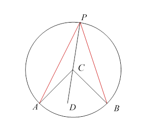
Given a chord $AB$ of a circle, the angle $APB$ for any point $P$ on the circle above the chord is twice the angle $ACB,$ where $C$ is the center of the circle. This follows from triangles $APC,BPC$ being isosceles, so the exterior angle $ACD$ (which is the sum of the two other interior angles)is twice the angle $APC.$ Hence angle $APB$ is half of the fixed angle $ACB,$ independent of where $P$ is on the upper part of the circle.

Hence the equipotentials are all the circles through the two points, except that if the arc above the two points is at potential $\theta ,$ the arc of the same circle below the two points is at potential $\theta -\pi .$ (Note: not $\pi -\theta .$ ) We’ve highlighted this for the circle having the two points as ends of a diameter.

The Split Pipe Problem

This is Jackson problem 2.13, perfect for our equipotentials.

A circular conducting pipe is actually two half pipes held together with a thin layer of insulator at the ends of a horizontal diameter, at $\pm b.$

We’ve switched from $a$ to $b$ to coincide with Jackson’s notation.

The top half is held at potential $V_1,$ the bottom half at $V_2.$ Find the potential inside. We’ll put in those potential values at the end, for now we’ll take

$$\phi \left(z\right)=\mathrm{Im}\ln \left(\frac{z-b}{z+b}\right).$$

Recall $z-b=r_1{e}^{i{\theta }_1},z+b=r_2{e}^{i{\theta }_2}$ so $\phi \left(z\right)={\theta }_1-{\theta }_2.$

To put this slightly differently, if we write

$$\left(\frac{z-b}{z+b}\right)=A{e}^{i\left({\theta }_1-{\theta }_2\right)}=A\cos \left({\theta }_1-{\theta }_2\right)+iA\sin \left({\theta }_1-{\theta }_2\right),$$

then

$$\tan \phi \left(z\right)=\tan \left({\theta }_1-{\theta }_2\right)=\mathrm{Im}\left(\frac{z-b}{z+b}\right)/\mathrm{Re}\left(\frac{z-b}{z+b}\right).$$

So the potential is the arctan of the ratio of the imaginary part to the real part of $\left(\frac{z-b}{z+b}\right).$

A trick for finding this easily is to multiply both numerator and denominator by the complex conjugate of the denominator: this gives a real denominator, so it plays no role in determining the ratio of real to imaginary parts, and the numerator becomes

$\left(z-b\right)\left(z*+b\right)={\left|z\right|}^2-b^2+b\left(z-z*\right).$

Writing $z=\rho e^{i\theta }$ in this expression, and separating out its real and imaginary parts, we immediately find

$$\phi \left(z\right)=\mathrm{Im}\ln \left(\frac{z-b}{z+b}\right)={\tan }^{-1}\left(\frac{2b\rho \sin \theta }{{\rho }^2-b^2}\right).$$

Looking at small values of $\rho ,$ we note that this potential is negative in the upper half plane, so to link up with Jackson’s problem 2.13 (and his angle $\varphi =\left(\pi /2\right)-\theta$ ) we must switch the sign.

A final adjustment: Our result is equal to $\pi /2$ on the top half of the cylinder (see figure), $-\pi /2$ on the bottom half. But we want something equal to $V_1$ on the top, $V_2$ on the bottom. It's easy to verify the correct expression is

$$\frac{V_1+V_2}{2}+\left(\frac{V_1-V_2}{\pi }\right){\tan }^{-1}\left(\frac{2b\rho \sin \theta }{b^2-{\rho }^2}\right).$$

Exercise: What about the potential outside the pipe? Sketch some field lines, inside and outside, to guide your thinking.

Charged Quadrants

Again we'll look at a cut circular pipe, but this time just separate off one-quarter of the circle.

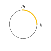
Suppose the quadrant (in the complex plane representation) between positive real $b$ and pure imaginary $ib$ is at one potential, the other three-quarters of the circle at a different potential.

The obvious strategy is to think of angles based on the chord joining the two ends $b$ and $ib,$ so look at $\mathrm{Im}\ln \left(\frac{z-b}{z-ib}\right).$

The angle in a quadrant is $\pi /4$ (half the angle the chord subtends at the center of the circle).

This is by way of introduction to Jackson problem 2.14(b), in which all four quadrants are electrically insulated where they join, and alternate ones are at potentials $\pm V.$ We can achieve this by simply adding the opposite chord to the one above, giving the relevant function to be

$$\mathrm{Im}\ln \left(\frac{z-b}{z-ib}\cdot \frac{z+b}{z+ib}\right)=\mathrm{Im}\ln \left(\frac{z^2-b^2}{z^2+b^2}\right).$$

As in the example above, the strategy is to multiply top and bottom by the complex conjugate of the denominator, then take arctan of the ratio of imaginary and real parts of the consequent numerator.

That is, the numerator becomes

$$\left(z^2-b^2\right)\left(z^{*2}+b^2\right)=\left({\rho }^2{e}^{2i\theta }-b^2\right)\left({\rho }^2{e}^{-2i\theta }+b^2\right)={\rho }^4-b^4+2i{\rho }^2{b}^2\sin 2\theta ,$$

and Jackson’s result follows (as before, we need to switch the sign.)

Exercise: try plotting the field lines just from a few facts: what do they look like near the joins? In the center? What about along the axes? The lines $x=\pm y$ ?

After you've sketched it, compare with this.

Bipolar Coordinates

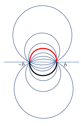
The two sets of circles discussed above are the basis for an orthogonal coordinate system labeled bipolar (yes, really). Here is a very nice plot from Wikipedia and the link

https://en.wikipedia.org/wiki/Bipolar_coordinates#/media/File:Iso1.svg

In the Wikipedia article, the parameter $\sigma$ is our $\theta ={\theta }_1-{\theta }_2,$ and $\tau =\ln \left(r_1/r_2\right).$

They write

$x+iy=ia\cot \frac{1}{2}\left(\sigma +i\tau \right).$

Exercise: Show this is equivalent to (from the beginning of this lecture)

$$w\left(x,y\right)=\ln \left(\frac{z-a}{z+a}\right)\text{.}$$

Making a 3D rotation of this diagram about the $y$ -axis generates the 3D toroidal coordinate system.

previous  index  next