previous  index  next 

18.  Electrostatics Using Spherical Coordinates: Spherical Harmonics

    Michael Fowler, UVa

Introduction

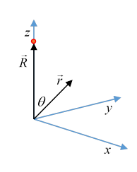
There are many situations on electrostatics, starting even with a single point charge at the origin, where the $\left(x,y,z\right)$ coordinates are a poor choice for analyzing the field$—$the potential depends only on radial distance $r,$ so obviously $r$ needs to be one of the coordinates.  The other two must fix location on the constant $r$ spherical surface. The standard choice is of course latitude and longitude, except that in physics we take the latitude angle $\theta$ to be zero at the north pole, increasing to $\pi /2$ at the equator and $\pi$ at the south pole.

The methods developed below for dealing with electric (and electromagnetic) fields in this coordinate system are often the most natural way of analyzing charge and current distributions, and the related electromagnetic radiation emanating from a bounded set of such oscillating charges/currents.  The same analysis works on all scales from atoms, through antennas and planetary phenomena, to galactic scales and above, where, admittedly, general relativistic effects will make the analysis more interesting (and we won’t cover that here).

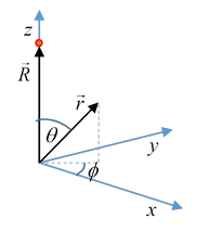
  Consider now the electric potential $\phi$ of a point charge not at the origin, but on the $z\text{-}$ axis : in $\left(r,\theta ,\varphi \right)$ coordinates, it clearly does not depend on $\varphi .$ in fact, a wide variety of systems have this azimuthal (meaning $\varphi$ - independent) symmetry, and $\left(r,\theta \right)$ are the natural coordinates for analyzing their electrostatic fields. 

Expressions for the common differential operators in $\left(r,\theta ,\varphi \right)$ can be found in my notes here.

Spherical Coordinates

In $\left(r,\theta ,\varphi \right)$ coordinates, Laplace's equation becomes:

$${\nabla }^2\phi =\frac{1}{r^2}\frac{\partial }{\partial r}{r}^2\frac{\partial \phi }{\partial r}+\frac{1}{r^2}\left\{\frac{1}{\sin \theta }\frac{\partial }{\partial \theta }\left(\sin \theta \frac{\partial \phi }{\partial \theta }\right)+\frac{1}{{\sin }^2\theta }\frac{{\partial }^2\phi }{\partial {\varphi }^2}\right\}=0.$$

As usual, we look for factorizable solutions (which, it later turns out, form a complete basis for all physically relevant solutions).  That is, we take

$\phi \left(r,\theta ,\varphi \right)=R\left(r\right)\Theta \left(\theta \right)\Phi \left(\varphi \right)$.

(Note: This is the standard notation, as in Wikipedia, Griffiths, etc.  Jackson, however, writes $\phi \left(r,\theta ,\varphi \right)=\frac{U\left(r\right)}{r}P\left(\theta \right)Q\left(\varphi \right).$ )

Making this substitution in the above equation, and then dividing by $R\Theta \Phi$ as usual (for instance, in quantum treatment of the hydrogen atom), gives a sum of three terms to be zero, the first term a function of $r$ only, the second of $\theta$ only, the third of $\varphi .$ (If you do need a reminder of how this works, details can be found here.)  These three terms must always add to zero: that is, for arbitrary values of $r,\theta ,\varphi .$  This can only happen if the three terms are in fact separately constant, otherwise we could just vary one of them to get a nonzero result.  (The individual constants of course add to zero.)

The simplest term to deal with is the azimuthal variation

$$\frac{1}{\Phi }\frac{d^2\Phi }{d{\varphi }^2}=\text{ constant}\text{.}$$

Since the potential is real and single valued, and $\varphi$ goes all the way around the spherical axis, we must have $\Phi \left(\varphi \right)$ a sum of terms $A_m\sin m\varphi +B_m\cos m\varphi$ for integer values of $m.$

The next term (in the $\left\{\right\}$ brackets in the differential equation) gives that $\Theta \left(\theta \right)$ must satisfy

$$\frac{1}{\sin \theta }\frac{d}{d\theta }\left(\sin \theta \frac{d\Theta }{d\theta }\right)-\frac{m^2\Theta }{{\sin }^2\theta }=-l\left(l+1\right)\Theta$$

where at this point we've used  ${\partial }^2\phi /\partial {\varphi }^2=-m^2\phi .$  Although at this stage $l\left(l+1\right)$ is an arbitrary constant, we write it this way using hindsight, because we’ll find the final equation, that for $R\left(r\right),$ becomes

$$\frac{d}{dr}\left(r^2\frac{dR}{dr}\right)=l\left(l+1\right)R,$$

so

$R=A{r}^l+B{r}^{-\left(l+1\right)}$.

We'll assume the field at the origin does not vary as a non-integral power of $r.$ 

Non-integral behavior would only happen in certain special geometries, such as conical conducting surfaces.  We encountered similar behavior in 2D for two conducting sheets at different potentials intersecting along a line with an arbitrary angle between them.

To study the equation for $\Theta \left(\theta \right)$ further, it's convenient to set $x=\cos \theta$, so the equation becomes

$$\left(\frac{d}{dx}\left(1-x^2\right)\frac{d}{dx}+l\left(l+1\right)-\frac{m^2}{1-x^2}\right)\Theta \left(x\right)=0.$$

Axially Symmetric Case:  Legendre’s Equation and Polynomials

In this section, we'll examine the axially symmetric case, $m=0,$ the differential equation becomes

$$\left(\frac{d}{dx}\left(1-x^2\right)\frac{d}{dx}+l\left(l+1\right)\right)\Theta \left(x\right)=0.$$

This is Legendre’s equation, and can be written as an eigenvalue equation, switching here to the standard notation $P_l\left(x\right)$:

$$-\left(\frac{d}{dx}\left(1-x^2\right)\frac{d}{dx}\right)P_l\left(x\right)=l\left(l+1\right)P_l\left(x\right)$$

on the interval $\pi \ge \theta \ge 0,$ that is, $-1\le x\le 1$. 

This is different from our previous operators in that the operator itself has singular points at the endpoints of the interval, so some discussion is required to establish that a complete orthogonal set of eigenfunctions can in fact be found. 

Notice first that for $l=0,$ possible independent solutions are $P_0\left(x\right)=1$ and $P_0\left(x\right)=\ln \left(1+x\right)-\ln \left(1-x\right).$ This second solution, although mathematically ok, is singular at the north and south poles, which are not special points$—$we could have set our coordinate system at any orientation.  So from now on we'll drop singular solutions (for any value of $l$ ).

For $l\ne 0,$ if we try a power series solution $P_l\left(x\right)={\displaystyle \sum _{j=0}^{\infty }{a}_j{x}^j},$ we find

$$a_{j+2}=\left[\frac{j\left(j+1\right)-l\left(l+1\right)}{\left(j+1\right)\left(j+2\right)}\right]a_j.$$

Evidently, the series terminates at $j=l.$ But what if $j$ is even and $l$ is odd?  Then the series will not terminate, the coefficients will asymptotically be equal, and the series will diverge at $x=1.$ This is not a physical solution of the original differential equation, so we conclude that if $l$ is even/odd, the series, a polynomial of degree $l,$ only includes even/odd powers of $x.$ 

The orthogonality of the different $P_l$ 's follows from the equation

$\left[l\left(l+1\right)-m\left(m+1\right)\right]{\displaystyle \underset{-1}{\overset{1}{\int }}{P}_l\left(x\right)P_m\left(x\right)dx}={\left[\left(P_l{P^{\prime }}_m-{P^{\prime }}_l{P}_m\right)\left(1-x^2\right)\right]}_{-1}^1.$ 

Since we are taking only nonsingular solutions, the right-hand side is zero.

We Could Have Found These Polynomials Using Schmidt Orthogonalization...

We've just shown that the $P_l\left(x\right)$ are a set of orthogonal polynomials in $x$ on the interval $\left(-1,1\right).$ 

But the standard Schmidt orthogonalization procedure applied to $1,x,x^2,\dots$  generates a unique set of orthogonal polynomials, so these have to be the $P_l$ 's , apart from normalization.   

Warning!  In contrast to orthogonal sets of functions we've previously encountered (such as Fourier series), the Legendre polynomials, by tradition, are not defined to be orthonormal: their normalization is defined by

$$P_l\left(1\right)=1.$$ 

The reason for this normalization convention will soon become evident.

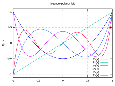
Here are plots of the first few $P_l$ 's (from Wikipedia).

From the Schmidt process plus normalization

$\begin{array}{l}{P}_0\left(x\right)=1\\ P_1\left(x\right)=x\\ P_2\left(x\right)=\frac{1}{2}\left(3x^2-1\right)\\ P_3\left(x\right)=\frac{1}{2}\left(5x^3-3x\right)\end{array}$

Rodrigues' Formula

Rodrigues discovered a very neat formula for generating the polynomials without having to go up the Schmidt ladder:

$$P_l\left(x\right)=\frac{1}{2^{l}l!}\frac{d^l}{d{x}^l}{\left(x^2-1\right)}^l.$$

It's straightforward to prove that  $P_l\left(x\right)$ defined in this way is a solution of the differential equation, and that the different $P_l$ ’s are orthogonal to each other. 

Exercise:  do it!

Therefore, since they are polynomials of the appropriate order, and mutually orthogonal, they must be the same as those found by successive orthogonalization, apart from normalization.   Rodrigues' prefactor ensures the standard normalization $P_l\left(1\right)=1.$ With this requirement, the $P_l$ 's are not orthonormal, in fact (as can be proved from Rodrigues' formula)

$${\displaystyle \underset{-1}{\overset{1}{\int }}{P}_l\left(x\right)P_m\left(x\right)dx}=\frac{2}{2l+1}{\delta }_{lm}.$$

They have alternating parity:

$P_l\left(-x\right)={\left(-1\right)}^l{P}_l\left(x\right).$

The Potential from a Point Charge in Legendre Polynomials: the Generating Function

The general axially symmetric (meaning $m=0$) solution of the Laplace equation, ${\nabla }^2\phi \left(r,\theta \right)=0,$ is

$\phi \left(r,\theta \right)={\displaystyle \sum _{l=0}^{\infty }\left(a_l{r}^l+b_l{r}^{-l-1}\right)P_l\left(\cos \theta \right)}.$

As a preliminary exercise, we take a unit charge on the $z\text{-}$ axis at $\overrightarrow{R}=\left(0,0,R\right).$   

Then the solution of ${\nabla }^2\phi =0$ in the region $\left|\overrightarrow{r}\right|<R$ must have the form (dropping the $1/4\pi {\epsilon }_0$, we're just doing math here, and we don’t want to clutter it up) :

$$\phi \left(\overrightarrow{r}\right)=\frac{1}{\left|\overrightarrow{r}-\overrightarrow{R}\right|}=\frac{1}{\sqrt{r^2+R^2-2rR\cos \theta }}={\displaystyle \sum _{l=0}^{\infty }{a}_l{r}^l{P}_l\left(\cos \theta \right)}.$$

(The $b_l$ ’s in the more general expansion given above have to all be zero, since $\phi$ is not singular at the origin$—$it’s just from the one charge, which is not at the origin.)

We can now find the $a_l$ ’s by setting $\theta =0$ and Taylor expanding:

$$\frac{1}{\left|\overrightarrow{r}-\overrightarrow{R}\right|}=\frac{1}{r-R}=\frac{1}{R}\left(1+\left(\frac{r}{R}\right)+{\left(\frac{r}{R}\right)}^2+\dots \right)$$

Therefore,

$$\frac{1}{\sqrt{r^2+R^2-2rR\cos \theta }}=\frac{1}{R}{\displaystyle \sum _{l=0}^{\infty }{\left(\frac{r}{R}\right)}^l{P}_l\left(\cos \theta \right)},r<R.$$

It's now evident why the normalization $P_l\left(1\right)=1$ is a good choice!

The function on the left is called the generating function of the Legendre polynomials.  (A generating function is a function of two variables: when it is expressed as a power series in one of the variables, the successive coefficients are the functions of the other variable we’re generating.)

An exactly similar argument, based on the nondivergent behavior of $\phi \left(r,\theta \right)$ at infinity, gives

$$\frac{1}{\sqrt{r^2+R^2-2rR\cos \theta }}=\frac{1}{r}{\displaystyle \sum _{l=0}^{\infty }{\left(\frac{R}{r}\right)}^l{P}_l\left(\cos \theta \right)},r>R.$$

You will often see these two formulas combined and written

$$\frac{1}{\left|\overrightarrow{r}-\overrightarrow{R}\right|}=\frac{1}{\sqrt{r^2+R^2-2rR\cos \theta }}=\frac{1}{r_{>}}{\displaystyle \sum _{l=0}^{\infty }{\left(\frac{r_{<}}{r_{>}}\right)}^l{P}_l\left(\cos \theta \right)}.$$

Using the Generating Function to Find Recursion Relations among Legendre Polynomials

In this section, to make the equations easier to read, we'll go back to the notation $\cos \theta =x,$ and also take $R=1$ (in the equation at the end of the last section).  Then, writing the generating function as $G\left(x,r\right),$ we have

$$G\left(x,r\right)=\frac{1}{\sqrt{1-2xr+r^2}}={\displaystyle \sum _{l=0}^{\infty }{r}^l{P}_l\left(x\right)}.$$

(Just repeating the equation for the case $r<1$ in the previous section.)

We can find recursion relations among the polynomials easily by differentiating the generating function with respect to its variables, then matching coefficients in the power series.

First, differentiating $G\left(x,r\right)$ with respect to $r,$ 

$$\frac{\partial G\left(x,r\right)}{\partial r}=\frac{x-r}{{\left(1-2xr+r^2\right)}^{3/2}},$$

or

$$\left(1-2xr+r^2\right)\frac{\partial G\left(x,r\right)}{\partial r}=\left(x-r\right)G\left(x,r\right).$$

Now writing this in terms of the polynomials,

$\left(1-2xr+r^2\right){\displaystyle \sum _{n=0}^{\infty }l{r}^{l-1}{P}_l\left(x\right)}=\left(x-r\right){\displaystyle \sum _{l=0}^{\infty }{r}^l{P}_l\left(x\right)}.$

Bonnet's Formula

Comparing coefficients of $r^l$ on the two sides we find

$\left(l+1\right)P_{l+1}-2xl{P}_l+\left(l-1\right)P_{l-1}=x{P}_l-P_{l-1},$

giving Bonnet's formula:

$\left(l+1\right)P_{l+1}-\left(2l+1\right)x{P}_l+l{P}_{l-1}=0.$

Notice that Bonnet’s formula enables a recursive method for successively constructing the polynomials: starting with $P_0=1,P_1=x$ we can generate them all.  

Bonnet's formula is also useful for finding ${\displaystyle \int x{P}_l{P}_{m}dx,}$ evidently only nonzero for $m=\pm l.$ (This is relevant for transitions between atomic angular momentum states induced by an external electric field.)

Finally, using Bonnet's formula it's easy to find the value of the (even) polynomials at the origin:

$$P_{2l}\left(0\right)=\frac{2l-1}{2l}{P}_{2l-2}\left(0\right)=\frac{\left(2l-1\right)\left(2l-3\right)\left(2l-5\right)\cdots 1}{2l\left(2l-2\right)\left(2l-4\right)\cdots 2}.$$

Recursion Relations Including Derivatives

More recursion relations are generated by differentiating $G\left(x,r\right)$ with respect to $x$

$$\left(1-2xr+r^2\right)\frac{\partial G\left(x,r\right)}{\partial x}=rG\left(x,r\right),$$

and equating the coefficient of $r^{l+1}$ on the two sides, to find

${P^{\prime }}_{l+1}-2x{P^{\prime }}_l+{P^{\prime }}_{l-1}=P_l.$

Subtracting $\left(2l+1\right)$ times this equation from twice the differential of Bonnet's equation, $\left(l+1\right)P_{l+1}-\left(2l+1\right)x{P}_l+l{P}_{l-1}=0$ gives

${P^{\prime }}_{l+1}-{P^{\prime }}_{l-1}=\left(2l+1\right)P_l.$

Putting this with

${P^{\prime }}_{l+1}+{P^{\prime }}_{l-1}=P_l+2x{P^{\prime }}_l,$

adding and subtracting give:

$\begin{array}{l}{P^{\prime }}_{l+1}\left(x\right)=\left(l+1\right)P_l\left(x\right)+x{P^{\prime }}_l\left(x\right),\\ {P^{\prime }}_{l-1}\left(x\right)=-l{P}_l\left(x\right)+x{P^{\prime }}_l\left(x\right).\end{array}$

We can actually use these recursion relations to prove that the polynomials do indeed satisfy Legendre's equation: here we go.

Taking the top equation of the two, but shift the index down by one, to get

${P^{\prime }}_l\left(x\right)=l{P}_{l-1}\left(x\right)+x{P^{\prime }}_{l-1}\left(x\right),$

Now add this to $x$ times the bottom equation,

$x{P^{\prime }}_{l-1}\left(x\right)+{P^{\prime }}_l\left(x\right)=-xl{P}_l\left(x\right)+x^2{P^{\prime }}_l\left(x\right)+l{P}_{l-1}\left(x\right)+x{P^{\prime }}_{l-1}\left(x\right),$

or

$\left(1-x^2\right){P^{\prime }}_l\left(x\right)=-xl{P}_l\left(x\right)+l{P}_{l-1}\left(x\right),$

Then take the derivative,

${\left(\left(1-x^2\right){P^{\prime }}_l\left(x\right)\right)}^{\prime }=-l{P}_l\left(x\right)-xl{P^{\prime }}_l\left(x\right)+l{P^{\prime }}_{l-1}\left(x\right),$

and finally, using ${P^{\prime }}_{l-1}\left(x\right)=-l{P}_l\left(x\right)+x{P^{\prime }}_l\left(x\right),$ we find

${\left(\left(1-x^2\right){P^{\prime }}_l\left(x\right)\right)}^{\prime }+l\left(l+1\right)P_l\left(x\right)=0,$

checking that the Legendre polynomials generated this way satisfy Legendre's equation$—$which of course we knew all along, since we began with a generating function satisfying Laplace's equation in the relevant region, so expanding ${\nabla }^2\phi$ in powers of $r,$ each term must satisfy it.

One final point:  the formula

${P^{\prime }}_{l+1}-{P^{\prime }}_{l-1}=\left(2l+1\right)P_l$

can be used to evaluate

${\displaystyle \underset{0}{\overset{1}{\int }}{P}_l\left(x\right)dx,}$

since we found the values of the polynomials at $x=0$ above.  (Notice the integral must be zero for an even polynomial, since it's orthogonal to $P_0=1.$ )

General Spherical Harmonics

It’s time to move from azimuthal symmetry to harmonics depending on both $\theta$ and $\varphi ,$ necessary in describing the electric potential from more general charge distributions.

So we’re back to

$$\left(\frac{d}{dx}\left(1-x^2\right)\frac{d}{dx}+l\left(l+1\right)-\frac{m^2}{1-x^2}\right)\Theta =0$$

with $l,m$ integers.  It turns out that the solutions are

$$P_l^m\left(x\right)={\left(-1\right)}^m{\left(1-x^2\right)}^{m/2}\frac{d^m}{d{x}^m}{P}_l\left(x\right)$$

and the spherical harmonics are defined as

$$Y_l^m\left(\theta ,\phi \right)=\sqrt{\frac{2l+1}{4\pi }\frac{\left(l-m\right)!}{\left(l+m\right)!}}{P}_l^{\left|m\right|}\left(\cos \theta \right)e^{im\varphi },-l\le m\le l.$$

These are orthonormal (from the corresponding property of the Legendre polynomials)

${\displaystyle \underset{0}{\overset{2\pi }{\int }}d\varphi }{\displaystyle \underset{0}{\overset{\pi }{\int }}\sin \theta d\theta Y_{l^{\prime }}^{m^{\prime }}*\left(\theta ,\varphi \right)Y_l^m\left(\theta ,\varphi \right)}={\delta }_{l^{\prime }l}{\delta }_{m^{\prime }m},$

and complete:

${\displaystyle \sum _{\mathcal{l}=0}^{\infty }{\displaystyle \sum _{m=-\mathcal{l}}^{\mathcal{l}}{Y}_{\mathcal{l}}^m*\left({\theta }^{\prime },{\varphi }^{\prime }\right)Y_{\mathcal{l}}^m\left(\theta ,\varphi \right)}}=\delta \left(\varphi -{\varphi }^{\prime }\right)\delta \left(\cos \theta -\cos {\theta }^{\prime }\right),$

nontrivial to prove, see for example Byron and Fuller for a proof.

The general solution of ${\nabla }^2\phi =0$ can be written as

$\phi \left(r,\theta ,\varphi \right)={\displaystyle \sum _{l=0}^{\infty }{\displaystyle \sum _{m=-l}^l\left(a_{lm}{r}^l+b_{lm}{r}^{-l-1}\right)}{Y}_l^m\left(\theta ,\varphi \right)}.$

It is sometimes useful to borrow notation from quantum mechanics, and write these as $Y_l^m\left(\theta ,\varphi \right)\equiv \left|l,m\right.〉.$  Localized states on the surface of the sphere, and the corresponding delta function, can be written

$\left.〈{\theta }^{\prime },{\varphi }^{\prime }\right|\theta ,\varphi 〉=\delta \left(\cos {\theta }^{\prime }-\cos \theta \right)\delta \left({\varphi }^{\prime }-\varphi \right)$

and

$Y_l^m\left(\theta ,\varphi \right)=〈\theta ,\varphi \left|l,m\right.〉.$

(Note: the area measure on the unit sphere is $\sin \theta d\theta d\varphi =-d\left(\cos \theta \right)d\varphi .$ this is why the delta function has the form above. To check the sign's right, remember $\cos \theta$ decreases as a function of $\theta$ in $\left(0,\pi \right)$.)

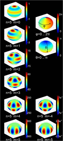
The spherical harmonics are eigenstates of vibration of a sphere, think a perfectly spherical balloon (pictures here from Wikimedia.).

They are also the angular patterns of wave functions for atomic orbitals, these being eigenstates of angular momentum, represented in quantum mechanics by an operator equivalent to ${\nabla }^2$ acting on the surface of a sphere.

Addition Theorem

An important identity is the so-called addition theorem for spherical harmonics:

$$P_l\left(\cos \gamma \right)=\frac{4\pi }{2l+1}{\displaystyle \sum _{m=-l}^l{Y}_l^m*\left({\theta }^{\prime },{\varphi }^{\prime }\right)Y_l^m\left(\theta ,\varphi \right)}$$

where $\cos \gamma =\cos \theta \cos {\theta }^{\prime }+\sin \theta \sin {\theta }^{\prime }\cos \left(\varphi -{\varphi }^{\prime }\right)$.

 

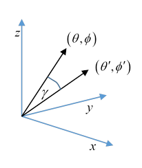
In other words, $\gamma$ is the angle between the direction $\left(\theta ,\varphi \right)$ and the direction $\left({\theta }^{\prime },{\varphi }^{\prime }\right),$ so $\cos \gamma$ is the dot product of two unit vectors of the form $\left(\sin \theta \cos \varphi ,\sin \theta \sin \varphi ,\cos \theta \right).$ 

Writing this as

$$P_l\left(\cos \gamma \right)=\frac{4\pi }{2l+1}{\displaystyle \sum _{m=-l}^l\left.〈{\theta }^{\prime },{\varphi }^{\prime }\right|l,m〉〈l,m}\left|\theta ,\varphi \right.〉,$$

notice that ${\displaystyle \sum _{m=-l}^l\left|l,m\right.〉}\left.〈l,m\right|$ is the identity operator within the eigenvalue $l$ subspace, hence clearly invariant under rotations, so we can conveniently re-orient to put ${\theta }^{\prime }=0,$ that is, along the $z$ axis. Now $Y_l^m\left(0,\varphi \right)$ is only nonzero for $m=0,$ otherwise the $e^{im\varphi }$ term would give a non-differentiable function along the axis. (Or, notice it has a factor ${\left(1-x^2\right)}^{\left|m\right|/2}$ )  

So, on the right-hand side, after re-orientation, only $m=0$ contributes, and the normalization condition

$$Y_{l0}=\sqrt{\frac{2l+1}{4\pi }}{P}_l\left(\cos \theta \right)$$

gives the result. 

Factorizing a Potential

This proves very useful in “factorizing” the potential between two charges,

$$\frac{1}{\left|\overrightarrow{r}-\overrightarrow{R}\right|}={\displaystyle \sum _{l=0}^{\infty }\frac{r_{<}^l}{r_{>}^{l+1}}{P}_l\left(\cos \gamma \right)}=4\pi {\displaystyle \sum _{l=0}^{\infty }\frac{1}{2l+1}\frac{r_{<}^l}{r_{>}^{l+1}}{\displaystyle \sum _{m=-l}^l{Y}_l^m*\left({\theta }^{\prime },{\varphi }^{\prime }\right)Y_l^m\left(\theta ,\varphi \right)}.}$$

Important!  As we shall soon see, the significance of this is that any charge distribution can be factored into monopole, dipole, quadrupole, etc., and this equation is telling us that the dipole component of a charge distribution generates a potential having dipole angular dependence, etc. As we’ll find later, this correspondence also holds between spherical components of oscillating charge distributions and components of the radiation emitted.

previous  index  next