19. Remarks on Some Azimuthally Symmetric Problems

    Michael Fowler, UVa

Split Sphere

Jackson revisits our old friend, the split sphere with the top and bottom halves at $\pm V$ respectively. Recall we found the potential on the axis as

$$\phi \left(r\right)=V\left[1-\frac{\left(r^2-a^2\right)}{r\sqrt{r^2+a^2}}\right]\left(\theta =0\right)$$ 

where here we’ve replaced $z$ with $r.$ Since we’re only in the region outside the sphere, $r>a,$ we can rearrange to get a factor

$$\phi \left(r\right)=V\left[1-\left(1-\frac{a^2}{r^2}\right){\left(1+\frac{a^2}{r^2}\right)}^{-1/2}\right]=V\left[\frac{3}{2}\frac{a^2}{r^2}-\frac{7}{8}\left(\frac{a^2}{r^2}\right)+\dots \right]$$ 

Going off axis is now trivial: from the uniqueness theorem, we know the answer must be

$$\phi \left(r,\theta \right)=V\left[\frac{3}{2}\frac{a^2}{r^2}{P}_1\left(\cos \theta \right)-\frac{7}{8}{\left(\frac{a^2}{r^2}\right)}^2{P}_3\left(\cos \theta \right)+\dots \right]$$ 

(For this particular case of the $\pm V$ hemispheres, only even powers of $r$ will enter, hence only odd powers of $P_n,$ remember the charge distribution itself has odd parity.)

On the sphere itself, $r=a,$ this polynomial expansion must equal the function equal to one on the top half hemisphere, minus one on the bottom half.

Therefore, the same series of coefficients must represent the potential inside the sphere, except that now ${\left(a/r\right)}^{\ell +1}$ is replaced by ${\left(r/a\right)}^{\ell }.$ 

General Axially Symmetric Charge Distribution on a Spherical Surface

 Suppose we have a spherical surface with charge density $\sigma \left(\theta \right),$ axially symmetric. This will cause a discontinuity in the radial electric field at the surface, but not in the potential.

So

$$\begin{array}{c}\phi \left(r,\theta \right)={\displaystyle \sum _{\ell =0}^{\infty }{c}_{\ell }{\left(\frac{r}{R}\right)}^{\ell }{P}_{\ell }\left(\cos \theta \right)r\le R,}\\ ={\displaystyle \sum _{\ell =0}^{\infty }{c}_{\ell }{\left(\frac{R}{r}\right)}^{\ell +1}{P}_{\ell }\left(\cos \theta \right)r\ge R.}\end{array}$$ 

The coefficients must match to ensure the continuity of the potential, but the slope is discontinuous:

$${\left[\frac{\partial {\phi }_{<}}{\partial r}-\frac{\partial {\phi }_{>}}{\partial r}\right]}_{r=R}=\frac{\sigma \left(\theta \right)}{{\epsilon }_0}.$$ 

This gives:

$${\displaystyle \sum _{\ell =0}^{\infty }\frac{c_{\ell }}{R}\left(2\ell +1\right)P_{\ell }\left(\cos \theta \right)}=\frac{\sigma \left(\theta \right)}{{\epsilon }_0}.$$ 

The orthogonality of the Legendre polynomials then gives

$$c_{\ell }=\frac{R}{2{\epsilon }_0}{\displaystyle \underset{0}{\overset{\pi }{\int }}d\theta \sin \theta \sigma \left(\theta \right)}{P}_{\ell }\left(\cos \theta \right).$$ 

Ring of Charge

Jackson's example is a ring of charge along latitude $\theta =\alpha ,$ total charge $q.$ 

The charge density function

$$\sigma \left(\theta \right)=\left(q/2\pi R\sin \alpha \right)\delta \left(\cos \theta -\cos \alpha \right)\delta \left(r\right).$$ 

(Check: ${\displaystyle \int \left(q/2\pi R\sin \alpha \right)\delta \left(\cos \theta -\cos \alpha \right)\delta \left(r\right)r^{2}drd\left(\cos \theta \right)}d\varphi =q.$ )

This gives $c_{\ell }=q{P}_{\ell }\left(\cos \alpha \right)/4\pi {\epsilon }_0.$ 

Therefore, the potential from the ring is:

$$\begin{array}{c}\phi \left(r,\theta \right)=\frac{q}{4\pi {\epsilon }_{0}R}{\displaystyle \sum _{\ell =0}^{\infty }{\left(\frac{r}{R}\right)}^{\ell }{P}_{\ell }\left(\cos \alpha \right)P_{\ell }\left(\cos \theta \right)r\le R,}\\ =\frac{q}{4\pi {\epsilon }_{0}r}{\displaystyle \sum _{\ell =0}^{\infty }{\left(\frac{R}{r}\right)}^{\ell }{P}_{\ell }\left(\cos \alpha \right)P_{\ell }\left(\cos \theta \right)r\ge R.}\end{array}$$ 

Note that as always the field with a certain angular symmetry is generated by a charge distribution having that symmetry.

Conical Hole or Sharp Point

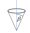
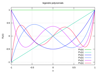
This is discussed in Jackson: the problem is the solution of $\overrightarrow{\nabla }\phi \left(r,\theta \right)=0$ with $\phi =0$ on a conical surface. Again we have azimuthal symmetry, the axis of the cone is $\theta =0,x=1$ and Legendre's equation is still valid.  However, we must now have $\phi =0$ for all points having the angle $\theta =\beta ,$ the angle of the cone.

Noticing from the graph below that the closest zero to $x=1$ gets closer and closer as $\ell$ increase, we can put it at $\beta$ if we choose a non-integral (in general) value of $\ell ,$ a solution of the form $r^{\nu }{P}_{\nu }\left(\cos \theta \right)$ with the right boundary condition, $P_{\nu }\left(\cos \beta \right)=0.$  

This generalized solution of Legendre's equation (and hence of ${\nabla }^2\phi =0$ )  is called a Legendre function of the first kind of order $\nu .$ 

From the graph, if $\beta =30$ degrees, so $x=\sqrt{3}/2,$ in the conical hole the field near the origin will be approximately of order $r^4.$ 

previous  index  next