21. Cylindrical Symmetry: Bessel Functions

    Michael Fowler, UVa

Introduction

The Bessel functions are solutions to Laplace’s equation in cylindrical coordinates $\rho ,\varphi ,z,$ that is:

$\begin{array}{c}{\nabla }^2\phi =\frac{1}{\rho }\frac{\partial }{\partial \rho }\left(\rho \frac{\partial \phi }{\partial \rho }\right)+\frac{1}{{\rho }^2}\frac{{\partial }^2\phi }{\partial {\varphi }^2}+\frac{{\partial }^2\phi }{\partial z^2}\\ =\frac{{\partial }^2\phi }{\partial {\rho }^2}+\frac{1}{\rho }\frac{\partial \phi }{\partial \rho }+\frac{1}{{\rho }^2}\frac{{\partial }^2\phi }{\partial {\varphi }^2}+\frac{{\partial }^2\phi }{\partial z^2}=0.\end{array}$ 

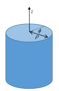
The usual separation of variables routine leads to solutions

$\phi \left(\rho ,\varphi ,z\right)=R\left(\rho \right)\Phi \left(\varphi \right)Z\left(z\right)$ 

with

$\begin{array}{c}\frac{d^{2}Z\left(z\right)}{d{z}^2}-k^{2}Z=0,\\ \frac{d^2\Phi \left(\varphi \right)}{d{\varphi }^2}+{\nu }^2\Phi =0,\\ \frac{d^{2}R\left(\rho \right)}{d{\rho }^2}+\frac{1}{\rho }\frac{dR\left(\rho \right)}{d\rho }+\left(k^2-\frac{{\nu }^2}{{\rho }^2}\right)R\left(\rho \right)=0.\end{array}$ 

The first two equations are of course simple: For positive $k^2,$ the solutions for $Z\left(z\right)$ will be exponentials.

For negative $k^2,$ $Z\left(z\right)$ is oscillatory, $e^{\pm ik\text{}z},\sin kz,$ etc.  

To ensure a single-valued potential, the equation for the angular variation, $\Phi \left(\varphi \right)$,  must have solutions $e^{\pm i\nu \varphi },$ with $\nu$ an integer.

Bessel Functions

For the positive $k^2$ case (often called hyperbolic behavior in the $z$ direction) the change of variable $x=k\rho$ puts the radial equation into what is the standard Bessel form:

$\frac{d^{2}R}{d{x}^2}+\frac{1}{x}\frac{dR}{dx}+\left(1-\frac{{\nu }^2}{x^2}\right)R=0,x=k\rho .$ 

In contrast to the Legendre polynomials for the spherical case, these Bessel functions are infinite series.

The Bessel equation is second-order, so for given $\nu$ there are two independent solutions.

First look at the equation near the origin: the 1 in the $\left(1-{\left(\nu /x\right)}^2\right)$ term can be dropped in the limit $x\to 0,$ and the solutions are then proportional to $x^{\nu },x^{-\nu }.$ Now look far away: the ${\nu }^2/x^2$ is negligible, and solutions look like combinations of $x^{-1/2}\sin x,x^{-1/2}\cos x.$ 

(By the way, this $x^{-1/2}$ amplitude is just what we need for propagating waves in two dimensions, discussed next semester, because the wave energy goes as the square of the amplitude, so as the wave goes outwards the same total energy crosses successive circles (or cylindrical surfaces) of circumference $2\pi r.$ )

Here are plots of those solutions which are well-behaved at the origin, with the standard normalization.

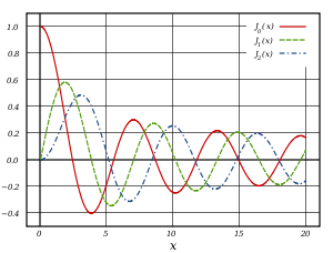
Behavior near the origin and far away:

$\begin{array}{l}{J}_{\nu }\left(x\right)=\frac{1}{\Gamma \left(\nu +1\right)}{\left(\frac{x}{2}\right)}^{\nu }+\cdots ,\\ J_{\nu }\left(x\right)\to \sqrt{\frac{2}{\pi x}}\cos \left(x-\frac{\nu \pi }{2}-\frac{\pi }{4}\right).\end{array}$ 

These $J_{\nu }\left(x\right)$ are called cylindrical Bessel functions.

The behavior goes from power law to oscillation in the region $x\sim \nu .$ 

In fact, it's not difficult to find the exact solution as a series.  Trying a solution $x^{\lambda }\left(1+c_{1}x+c_2{x}^2+\cdots \right)$ in the differential equation, we find $\lambda =\pm \nu$, coefficients of odd powers are zero, and successive coefficients of even powers have simple ratios, the result for the nonsingular solution is

$J_{\nu }\left(x\right)={\left(\frac{x}{2}\right)}^{\nu }{\displaystyle \sum _{n=0}^{\infty }\frac{{\left(-1\right)}^n}{\Gamma \left(n+1\right)\Gamma \left(n+\nu +1\right)}{\left(\frac{x}{2}\right)}^{2n}}.$ 

(Recall $\Gamma \left(n+1\right)=n!$ )

The Neumann Function

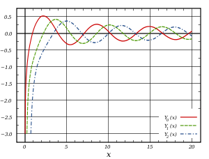
(Graph from Wikipedia Commons)

For integer $\nu =n$, $J_{-n}\left(x\right)={\left(-1\right)}^n{J}_n\left(x\right)$ so we have only found one solution.

Exercise: Prove the above equality be writing the first few terms in the series, and using properties of the factorial/gamma function.

The other solution is called the Neumann function, defined as

$N_{\nu }\left(x\right)=\frac{J_{\nu }\left(x\right)\cos \nu \pi -J_{-\nu }\left(x\right)}{\sin \nu \pi },$ 

it remains independent even as $\nu$ becomes integral (details in Stone and Goldbart, p 279).

The Neumann function is singular at the origin:

$N_{\nu }\left(x\right)=\frac{1}{\pi }{\left(\frac{x}{2}\right)}^{-\nu }\Gamma \left(\nu \right)+\cdots$ 

but similar to $J_{\nu }\left(x\right)$ far away:

$N_{\nu }\left(x\right)\to \sqrt{\frac{2}{\pi x}}\sin \left(x-\frac{\nu \pi }{2}-\frac{\pi }{4}\right).$ 

The transition from small $x$ to large $x$ behavior again takes place when $x\sim \nu .$ 

Hankel Functions (in and out waves at infinity)

The Bessel functions of the third kind, called Hankel functions, are the linear combinations:

$\begin{array}{l}{H}_{\nu }^{\left(1\right)}\left(x\right)=J_{\nu }\left(x\right)+i{N}_{\nu }\left(x\right)\\ H_{\nu }^{\left(2\right)}\left(x\right)=J_{\nu }\left(x\right)-i{N}_{\nu }\left(x\right)\end{array}$ 

Evidently, these behave at large $x$ as outgoing and incoming waves:

$H_{\nu }^{\left(1\right),\left(2\right)}\to \sqrt{\frac{2}{\pi x}}{e}^{\pm i\left(x-\nu \pi /2-\pi /4\right)}.$ 

Modified Bessel Functions $I_{\nu }\left(x\right),K_{\nu }\left(x\right)$ (exponential at infinity)

If in solving ${\nabla }^2\phi =0$ in a cylinder the given boundary conditions require oscillatory behavior in the $z\text{-}$ direction, then $k^2<0$ and the Bessel functions have pure imaginary argument.  It is convenient to introduce new notation in this case, so we define

$\begin{array}{l}{I}_{\nu }\left(x\right)=i^{-\nu }{J}_{\nu }\left(ix\right),\\ K_{\nu }\left(x\right)=\frac{1}{2}\pi i^{\nu +1}{H}_{\nu }^{\left(1\right)}\left(ix\right),\end{array}$ 

 real functions for real $x,\nu .$ 

Exercise:  check the behavior of these functions for very small and very large argument by substituting $ix$ in the results above for Bessel and Hankel functions. In particular, note that $I$ has exponential increase, $K$ exponential decrease at large $x,$ apart from the usual $x^{-1/2}$ term.

Radial Equation Inside a Grounded Cylinder

Since the interior of the cylinder includes the radial origin, this solution must be made up of $J_{\nu }\left(x\right)\text{'s.}$ 

The $\nu$ will in fact be the integer $m$ from the azimuthal equation. 

Furthermore, the solution is identically zero on the cylinder $\rho =a,$ so the only possibilities are the $J_{\nu }\left(k_{\nu n}\rho \right)$ where $k_{\nu n}={\alpha }_{\nu n}/a,$ and the ${\alpha }_{\nu n}$ are the zeroes of the Bessel function, $J_{\nu }\left({\alpha }_{\nu n}\right)=0.$ 

These zeroes are of course tabulated, and the first few ${\alpha }_{\nu n}$ are given in Jackson: the spacing soon tends to $\pi$:

$\begin{array}{l}\nu =0:{\alpha }_{01}=2.4,{\alpha }_{02}=5.5,{\alpha }_{03}=8.7,\dots \\ \nu =1:{\alpha }_{11}=3.8,{\alpha }_{12}=7.0,{\alpha }_{13}=10.2,\dots \\ \nu =2:{\alpha }_{21}=5.1,{\alpha }_{22}=8.4,{\alpha }_{23}=11.6,\dots \end{array}$

You can see these, approximately, on the graphs of the first $J_{\nu }\left(x\right)$ 's given above.

The Fourier-Bessel Series

Suppose now we have to solve ${\nabla }^2\phi =0$ inside a cylinder, going to zero at the walls $\rho =a.$ 

We shall show that the set of functions $\sqrt{\rho }{J}_{\nu }\left({\alpha }_{\nu n}\rho /a\right)$ are an orthogonal set on $0\le \rho \le a.$  An expansion of an arbitrary function in terms of these is called a Fourier-Bessel series.

The equation satisfied by $J_{\nu }\left(k\rho \right)$ is:

$\frac{1}{\rho }\frac{d}{d\rho }\left(\rho \frac{d{J}_{\nu }\left(k\rho \right)}{d\rho }\right)+\left(k^2-\frac{{\nu }^2}{{\rho }^2}\right)J_{\nu }\left(k\rho \right)=0.$ 

Take any $k_1,k_2$ to be any of the $k_{\nu n}={\alpha }_{\nu n}/a,$ remember the ${\alpha }_{\nu n}$ are the zeroes of $J_{\nu },$ so $J_{\nu }\left(k_{1}a\right)=J_{\nu }\left(k_{2}a\right)=0.$ 

Then

$\begin{array}{l}\rho \frac{d}{d\rho }\left(\rho \frac{d{J}_{\nu }\left(k_1\rho \right)}{d\rho }\right)+\left(k_1^2{\rho }^2-m^2\right)J_{\nu }\left(k_1\rho \right)=0,\\ \rho \frac{d}{d\rho }\left(\rho \frac{d{J}_{\nu }\left(k_2\rho \right)}{d\rho }\right)+\left(k_2^2{\rho }^2-m^2\right)J_{\nu }\left(k_2\rho \right)=0.\end{array}$ 

Now multiply the first equation by $J_{\nu }\left(k_2\rho \right)$, the second by $J_{\nu }\left(k_1\rho \right)$ and subtract to get

$\left(k_2^2-k_1^2\right)\rho J_{\nu }\left(k_1\rho \right)J_{\nu }\left(k_2\rho \right)=\frac{d}{d\rho }\left(J_{\nu }\left(k_2\rho \right)\rho \frac{d{J}_{\nu }\left(k_1\rho \right)}{d\rho }-J_{\nu }\left(k_1\rho \right)\rho \frac{d{J}_{\nu }\left(k_2\rho \right)}{d\rho }\right).$ 

 Integrating from $\rho =0$ to $\rho =a,$ the term on the right is zero at both ends, so

$\left(k_2^2-k_1^2\right){\displaystyle \underset{0}{\overset{a}{\int }}\rho J_{\nu }\left(k_1\rho \right)J_{\nu }\left(k_2\rho \right)d\rho }=0.$ 

Notice that this integral includes a weight function $\rho$.  To construct an orthonormal basis, we need also that

${\displaystyle \underset{0}{\overset{a}{\int }}\rho {\left[J_{\nu }\left(k_1\rho \right)\right]}^{2}d\rho }=\frac{a^2}{2}{\left[J_{\nu +1}\left(k_{1}a\right)\right]}^2.$ 

(Proving this requires recursion properties of the Bessel functions we'll discuss later.)

We can now expand an arbitrary function $f\left(\rho \right)$ equal to zero at $\rho =a$ on the interval $0\le \rho \le a$:

$f\left(\rho \right)={\displaystyle \sum _{n=1}^{\infty }{c}_{\nu n}{J}_{\nu }\left(k_{\nu n}\rho \right)}$ 

where

$c_{\nu n}=\frac{2}{R^2{J}_{\nu +1}^2\left(k_{\nu n}R\right)}{\displaystyle \underset{0}{\overset{a}{\int }}\rho f\left(\rho \right)J_{\nu }\left(k_{\nu n}\rho \right)d\rho .}$ 

This is the conventional Fourier-Bessel series, for functions vanishing at $\rho =a,$ that is, Dirichlet boundary conditions.

Another possible expansion is in functions whose derivatives vanish at the boundary, that is, $J_{\nu }\left(y_{\nu n}\rho /a\right)$ where ${J^{\prime }}_{\nu }\left(y_{\nu n}\right)=0.$  

But there’s more: if we replaced $k^2$ by $-k^2,$ the $Z\left(z\right)$ would be $\sin kz$ or $\cos kz.$ The Bessel equation would be changed to

$\frac{d^{2}R}{d{x}^2}+\frac{1}{x}\frac{dR}{dx}-\left(1+\frac{{\nu }^2}{x^2}\right)R=0$ 

and the solutions are called modified Bessel functions. These are exponentially growing or decaying functions, they’re really just Bessel functions with pure imaginary argument,

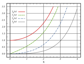
(Graph from Wikipedia Commons)

$\begin{array}{l}{I}_{\nu }\left(x\right)=i^{-\nu }{J}_{\nu }\left(ix\right)\\ K_{\nu }\left(x\right)=\frac{\pi }{2}{i}^{\nu +1}{H}_{\nu }^{\left(1\right)}\left(ix\right)\\ H_{\nu }^{\left(1\right)}=J_{\nu }+i{N}_{\nu }.\end{array}$ 

So what do the possible solutions of ${\nabla }^2\phi =0$ inside the cylinder look like? Obviously, that depends on the boundary conditions, but we can make one general remark. Recall from Earnshaw’s theorem that $\phi$ cannot have a minimum in the volume. This means that all three components cannot be of the oscillatory type. The $\varphi$ component must be oscillating (or constant) so the other two must be of opposite types. We can see this: if $k^2>0,$ the $z$ direction behavior is hyperbolic, the radial is oscillating; if $k^2<0$ the opposite is the case.

 Bessel Generating Function and Identities

The two-dimensional Helmholtz (wave) equation $\left({\nabla }^2+k^2\right)f\left(r,\varphi \right)=0$  has (nonsingular) solutions $e^{in\varphi }{J}_n\left(kr\right).$  Any other nonsingular solution to the wave equation should be expandable in terms of these functions, in particular a plane wave:

$e^{iky}=e^{ikr\sin \varphi }={\displaystyle \sum _{n=0}^{\infty }{c}_n{e}^{in\varphi }{J}_n\left(kr\right)}.$ 

In fact we'll show the $c_n$ are all equal to one, so  

$e^{ikr\sin \varphi }={\displaystyle \sum _{n=0}^{\infty }{e}^{in\varphi }{J}_n\left(kr\right)}.$ 

From this, we have

$J_n\left(x\right)=\frac{1}{2\pi }{\displaystyle \underset{0}{\overset{2\pi }{\int }}{e}^{-in\varphi +ix\cos \varphi }d\varphi .}$ 

Tip:  any time you come across an exponential of a trig function, you're probably dealing with a Bessel function!

The generating function is also often written (putting $e^{i\varphi }=t,kr=x$ )

$e^{\frac{x}{2}\left(t-\frac{1}{t}\right)}={\displaystyle \sum _{n=-\infty }^{\infty }{t}^n{J}_n\left(x\right).}$ 

Expanding the left-hand side and collecting powers of $t$ we eventually find

$e^{\frac{x}{2}\left(t-\frac{1}{t}\right)}={\displaystyle \sum _{n=-\infty }^{\infty }{t}^n\left[{\displaystyle \sum _{s=0}^{\infty }\frac{{\left(-1\right)}^s}{\Gamma \left(s+1\right)\Gamma \left(s+n+1\right)}{\left(\frac{x}{2}\right)}^{s+n}}\right]},$ 

the correct expression for the Bessel function, proving that the coefficients were indeed all equal to one, as assumed.  (OK, it was hindsight.)

From the expression for $J_n\left(x\right)$ and from the generating function, it's not difficult to find the recurrence relations

$\begin{array}{c}2{J^{\prime }}_n\left(x\right)=J_{n-1}\left(x\right)-J_{n+1}\left(x\right),\\ \frac{2n}{x}{J}_n\left(x\right)=J_{n-1}\left(x\right)+J_{n+1}\left(x\right).\end{array}$ 

Exercise:  do it! They both come from differentiation … but with respect to what?

Bessel Functions in Physics

If you look up Bessel functions in Jackson’s index, you’ll find that they’re going to appear many times in this course:  from cables and waveguides to diffraction to relativistic synchrotron radiation.  But they also appear in contexts not mentioned by Jackson. Consider, for example, transmitting information by modulating a carrier wave. Here’s an example from Quantum Electronics, by Amnon Yariv. Polarized light of a particular orientation is passed through a KDP crystal. The index of refraction $n$ can be varied linearly by an applied electric field. This means that for a light beam (frequency $\omega$ ) going through a given length of crystal, there will be a phase delay (or advance) proportional to the applied field, which could be oscillating at GHz, say a modulation frequency ${\omega }_m.$ Of course, ${\omega }_m\ll \omega .$  The outcoming electric field will therefore have amplitude

$E_{\text{out}}=A\cos \left(\omega t+\delta \sin {\omega }_{m}t\right)$

(Yariv p 314) where the modulation index $\delta$ is proportional to the modulating field multiplied by length of path and optical constants of the crystal. From the equation $e^{ikr\sin \varphi }={\displaystyle \sum _{n=0}^{\infty }{e}^{in\varphi }{J}_n\left(kr\right)}$ given above (both the real and imaginary parts), and using $J_{-n}\left(x\right)={\left(-1\right)}^n{J}_n\left(x\right),$ we can show that

$E_{\text{out}}=A\left[J_0\left(\delta \right)\cos \omega t+J_1\left(\delta \right)\cos \left(\omega +{\omega }_m\right)t-J_1\left(\delta \right)\cos \left(\omega -{\omega }_m\right)t+J_2\left(\delta \right)\cos \left(\omega +2{\omega }_m\right)t-\cdots \right]$

Remember $\omega \gg {\omega }_m,$ and ${\omega }_m$ can be slowly varying, that’s how the information is transmitted.  Now $\delta$ is proportional to the applied field strength, so we can set it to be 2.4048, the first zero of the Bessel function $J_0,$ and all the energy will then be in the information-carrying sidebands of the signal.