previous  index  next 

27.  Dielectrics I:  Polarization

    Michael Fowler, UVa

Introduction

We’ve reached Jackson section 4.3, he talks of “ponderable” media, which apparently means (from the dictionary) media other than the aether.  In other words, pretty much anything.  We’ll assume solids, possibly occasionally liquids, but no gases.

We've already discussed metals, which are solids containing highly mobile electrons in sufficient numbers that when a piece of metal is placed in a static electric field, these "free" electrons (meaning not bound locally in molecules, but they can’t get out of the solid) move to the surfaces until the interior of the metal is completely shielded from the field.

Solids containing no (or very few) free electrons are often referred to as dielectrics.  The electric field penetrates the solid (because not enough electrons can move to the surfaces to shield it out), and molecules inside the solid are distorted in response to the field$—$their bound electrons can move within the atom or molecule, so an external field can induce a dipole moment.  

Microscopically, of course, the electric field varies wildly on an atomic scale. When we talk about the electric field inside the dielectric, we mean the average electric field, meaning the field averaged over many atoms, but still over a region small by macroscopic standards, and small compared with the distances over which that field changes significantly.  We could take a spherical volume containing, say, 10,000 atoms, but give it a fuzzy edge, so there are no sudden jumps in enclosed charge or enclosed electric field on moving it a little.

What can we say about this averaged, or macroscopic, field inside a dielectric placed in an external field?  This is electrostatics, so we assume any distortions of molecules, etc., that took place as the external field was switched on have settled down. Obviously, the averaged field must satisfy

$\overrightarrow{\nabla }\times \overrightarrow{E}=0,$

because the work done on a charge as it moves along a path inside the solid is

${\displaystyle \underset{{\overrightarrow{r}}_1}{\overset{{\overrightarrow{r}}_2}{\int }}q\overrightarrow{E}\cdot \overrightarrow{dl}}$

and if this is nonzero around a closed path, we have a perpetual motion machine.

It follows that

$\overrightarrow{E}=-\overrightarrow{\nabla }\phi$

for both the microscopic (atomic scale) and the macroscopic (averaged) electric fields.

To make further progress, we need a plausible approximation to the distortion of the molecular charge distribution caused by an imposed electric field, and the new field generated by this distortion. 

Electric Polarization

We define the polarization $\overrightarrow{P}\left(\overrightarrow{r}\right)$ as the local induced dipole density.  Following Jackson, we assume the material is locally homogeneous, in general containing different molecules, each molecule having zero net charge, and in nonzero external field molecules of type $i$, with local density $n_i\left(\overrightarrow{r}\right),$ have mean polarization $〈{\overrightarrow{p}}_i〉$ (which we're taking to be linear in the imposed field) so the macroscopic polarization

$\overrightarrow{P}\left(\overrightarrow{r}\right)={\displaystyle \sum _i〈{\overrightarrow{p}}_i〉n_i\left(\overrightarrow{r}\right)}.$

Zangwill, by the way, points out that this is really oversimplified: with modern density functional quantum techniques, we can construct reasonably accurate maps of the charge density variations in a solid, and how they respond to an increasing imposed electric field.  A moment's thought will make clear that we can't really think of a polarized solid as a lattice of elementary dipoles, it's a solid, so there are valence bonds holding everything together, these bonds are electrons, they too will respond to the electric field.  Zangwill gives as an example a computed picture of an ionic crystal where some of the inner ionic orbits shift the opposite way in an external field, a result of exchange interactions with outer shell electrons.

Nevertheless, a dielectric in zero field has, on a macroscopic scale, the negative charge density exactly balancing the positive charge density, and on cranking up an applied field, the positive nuclei will move very slightly, the electron orbits will distort to cause an overall shift in the negative charge distribution in the direction opposite to the field, and, even though different electron orbit will move by different amounts, some even possibly negative, these are all small shifts and can be represented in total (on a scale of thousands of atoms or more) by an induced local dipole moment density. There is no need for higher moments or further refinement at the macroscopic scale. (Of course, if we want to predict theoretically a numerical value of the polarization induced by a given field, we'll need to do those difficult density functional theory calculations.  In this course, we'll just accept the experimentally determined value of the response.) It should perhaps be mentioned that in, say, a single crystal solid, the bound electrons might respond more easily in some particular direction of the applied field,  in which case the polarization $\overrightarrow{P}$ will in general not be parallel to the applied field $\overrightarrow{E}.$ We’ll see examples next semester in optical phenomena, for now we’ll assume the response is isotropic.

Incidentally, Zangwill points out (following Purcell) that just looking at a local charge pattern is not enough to figure out the local polarization, or dipole density. Consider for example a two-dimensional sodium chloride crystal, think of it as a checker board. Take one sodium ion (positive) and one of its four neighbor chlorine ions, they form a dipole. You can now cover the board with parallel dipoles, so it looks polarized. But we could have chosen any of the neighboring ions, we could equally see it polarized the opposite way!   

The point is, to find the direction of polarization, we need to take a finite piece of material, and see what's going on at the surfaces.  To remove ambiguity, we need to crank up the external field from zero. Even if, looking at only the interior, the polarization is not uniquely defined, the change in polarization is, so starting from zero provides a definite answer. At the same time,  the electrons will pile up to make some surfaces negatively charged, other sides will be depleted of electrons, and therefore positive.

A Polarized Dielectric Sphere with Zero External Field

To get some feeling for dielectric polarization, we'll begin with a toy example: a uniformly polarized sphere, no external applied field.  (This isn't entirely fantasy: there are materials called ferroelectrics, which do have inbuilt polarization. However, exposed to the atmosphere they tend to attract loose ions to neutralize the unbalanced surface charge.)

We'll represent this uniformly polarized sphere by taking a sphere of positive charge, radius $a,$ charge density $+\rho ,$ centered at the origin, superposed on an exactly similar sphere of negative charge, density $-\rho ,$ centered at a small displacement $-\overrightarrow{\delta }$ (so the dipole moment vector is in direction $+\overrightarrow{\delta }.$ )

From Gauss' theorem, the (spherically symmetric) electric field strength from the positively charged sphere is given by $4\pi r^{2}E=\left(4/3\right)\pi r^3\rho /{\epsilon }_0$, that is, inside the sphere the (radial) electric field

$${\overrightarrow{E}}_{\text{+ sphere}}\left(\overrightarrow{r}\right)=\frac{\rho \overrightarrow{r}}{3{\epsilon }_0},r<a,$$

 and outside it is

$$\overrightarrow{E}\left(\overrightarrow{r}\right)=\frac{1}{4\pi {\epsilon }_0}\cdot \frac{4}{3}\pi a^3\rho \cdot \frac{\widehat{\overrightarrow{r}}}{r^2}=\frac{a^3\rho }{3{\epsilon }_0}\cdot \frac{\widehat{\overrightarrow{r}}}{r^2},$$

corresponding to an (outside) potential

$$\phi \left(\overrightarrow{r}\right)=\frac{a^3\rho }{3{\epsilon }_0}\cdot \frac{1}{r}.$$

Creating the uniformly polarized sphere by putting together the fields from the positive and the negative spheres, we find the inside field of the polarized dielectric sphere is uniform,

$$\overrightarrow{E}\left(\overrightarrow{r}\right)=\frac{\rho \left(\overrightarrow{r}-\left(\overrightarrow{r}+\overrightarrow{\delta }\right)\right)}{3{\epsilon }_0}=\frac{-\rho \overrightarrow{\delta }}{3{\epsilon }_0},r<a,$$

and outside the potential is

$$\phi \left(\overrightarrow{r}\right)=\frac{a^3\rho }{3{\epsilon }_0}\overrightarrow{\delta }\cdot \overrightarrow{\nabla }\frac{1}{r}.$$

 Remember the polarization is defined as the dipole moment density, so it is

$\overrightarrow{P}=\rho \overrightarrow{\delta }.$

Hence the electric field inside the sphere is

$$\overrightarrow{E}\left(\overrightarrow{r}\right)=\frac{-\overrightarrow{P}}{3{\epsilon }_0},r<a,$$

and outside the potential is that of a dipole, moment $\overrightarrow{\mu },$ 

$$\phi \left(\overrightarrow{r}\right)=\frac{1}{4\pi {\epsilon }_0}\cdot \frac{\overrightarrow{\mu }\cdot \widehat{\overrightarrow{r}}}{r^2},\overrightarrow{\mu }=\frac{4}{3}\pi a^3\overrightarrow{P},r>a.$$

Exercise:  from the two superposed spheres shown above, locate the unbalanced charge, and sketch how that generates these fields and potentials.

Dielectric in a Field: Potential from Free Charges Plus Polarization

Turning now to the general case of a dielectric in an external field, and using the expression we just found for the electrostatic potential from a dipole, the total electric potential, including possible free charge density (meaning ordinary mobile charges, as in a conductor, not charges bound in molecules) is (summing over the induced elementary dipoles $\overrightarrow{P}\left(\overrightarrow{r^{\prime }}\right)d^3{r}^{\prime }$ )

$$\phi \left(\overrightarrow{r}\right)=\frac{1}{4\pi {\epsilon }_0}{\displaystyle \underset{\text{all space}}{\int }{d}^3{r}^{\prime }\left[\frac{{\rho }_{\text{free}}\left({\overrightarrow{r}}^{\prime }\right)}{\left|\overrightarrow{r}-{\overrightarrow{r}}^{\prime }\right|}+\overrightarrow{P}\left({\overrightarrow{r}}^{\prime }\right)\cdot {\overrightarrow{\nabla }}^{\prime }\left(\frac{1}{\left|\overrightarrow{r}-{\overrightarrow{r}}^{\prime }\right|}\right)\right]}.$$

Notice this integral is over all of space: the charge distribution ${\rho }_{\text{free}}\left({\overrightarrow{r}}^{\prime }\right)$ can be outside or inside the dielectric, and it is generating the initial electric field.  (For example, we could have a chunk of dielectric between two charged plates.)  The polarization contribution $\overrightarrow{P}\left({\overrightarrow{r}}^{\prime }\right)$ is of course entirely from the dielectric.

Now, integrating by parts (assuming zero contribution from infinity) gives

$$\phi \left(\overrightarrow{r}\right)=\frac{1}{4\pi {\epsilon }_0}{\displaystyle \underset{\text{all space}}{\int }{d}^3{r}^{\prime }\frac{1}{\left|\overrightarrow{r}-{\overrightarrow{r}}^{\prime }\right|}\left[{\rho }_{\text{free}}\left({\overrightarrow{r}}^{\prime }\right)-{\overrightarrow{\nabla }}^{\prime }\cdot \overrightarrow{P}\left({\overrightarrow{r}}^{\prime }\right)\right]}.$$

It is now evident that $-\overrightarrow{\nabla }\cdot \overrightarrow{P}\left(\overrightarrow{r}\right)$ is equivalent to a charge density.  (Notice the integral is over all of space:  this means it includes contributions from the rapid variation in polarization at the boundary of the dielectric.)

But how can we picture this internal charge density apparently generated by a spatially varying polarization?  It's easy to see with a one-dimensional model:  Imagine a lattice of equally spaced positive charges, and a displaced lattice of negative charges. Now suppose that on moving to the right, the negative charges we see are more and more displaced, meaning increasing negative polarization. Then the average spacing between them is greater than that between the fixed positive charges, and is given by how rapidly their displacement from the local positive charge is increasing, that is, by $\partial P_x/\partial x$.

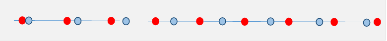
Over this interval, the positive charge density is clearly greater than the negative charge density.

Exercise:  Check this by drawing in little vectors for the local dipoles, they point backwards (so $\overrightarrow{P}$ is negative) for the above example, but increase in strength on moving to the right. Hence $-\overrightarrow{\nabla }\cdot \overrightarrow{P}\left(\overrightarrow{r}\right)$ is positive.

Exercise: Now consider a single point charge in an infinite uniform dielectric medium.  How is the medium polarized?  What is the polarization charge density $-\overrightarrow{\nabla }\cdot \overrightarrow{P}\left(\overrightarrow{r}\right)$?

Answer:  Yes, the medium is polarized, but since $\overrightarrow{P}\propto \overrightarrow{E},$ the polarization charge density, $-\overrightarrow{\nabla }\cdot \overrightarrow{P}\left(\overrightarrow{r}\right),$ is proportional to the divergence of the local field, so in fact zero except exactly on top of the single point charge. (Well, really fuzzed out over atomic distances.)  Of course, this is no longer true if the medium has a boundary.

It follows that the first Maxwell equation with a dielectric medium present is

$$\overrightarrow{\nabla }\cdot \overrightarrow{E}=\frac{1}{{\epsilon }_0}\left({\rho }_{\text{free}}-\overrightarrow{\nabla }\cdot \overrightarrow{P}\right).$$

But there's more: imagine a sphere of dielectric placed in a constant electric field. 

We'll go through a formal solution later, the result is it is uniformly polarized, so there is no $\overrightarrow{\nabla }\cdot \overrightarrow{P}$ term in the interior.

However, there is such a term at the surface: think of Gauss' theorem for a small pillbox, one surface outside the dielectric (where there's no material, so no polarization), one inside. 

In the mathematical limit of a thin pillbox, there is a delta function contribution to $\overrightarrow{\nabla }\cdot \overrightarrow{P}$ equal to the normal component of the polarization. This is also easy to see from our discussion of a uniformly polarized sphere: there is no free charge in that problem, the field is generated purely by the polarization$—$but not by the uniform internal polarization, only by the abruptly changing polarization at the surface.

Electric Displacement

Maxwell introduced the electric displacement $\overrightarrow{D}$ by

$\overrightarrow{D}={\epsilon }_0\overrightarrow{E}+\overrightarrow{P}$

from which

$\overrightarrow{\nabla }\cdot \overrightarrow{D}={\rho }_{\text{free}}.$

This field $\overrightarrow{D}$ is called the electric displacement because the $\overrightarrow{P}$ obviously arises from displacing charges, and Maxwell felt that the vacuum, thought of in those days as a medium itself and called the aether, had similar structure to a dielectric, and somehow charges were being displaced there too.  Of course, this turned out not to be the case, but the name stuck.  The ${\epsilon }_0$ makes the point that $\overrightarrow{D}$ is dimensionally different from $\overrightarrow{E}$, (well, in these SI units) even in a vacuum.

Why are we still bothering with this field $\overrightarrow{D}$?  It turns out to be useful: notice its divergence only comes from the free charges.  This sounds like a great idea$—$this is the "real" electric field from the real charges, right?  But not so fast$—$it's not conservative:  unlike $\overrightarrow{E},$ its curl isn't identically zero.

$\overrightarrow{\nabla }\cdot \overrightarrow{D}={\rho }_{\text{free}},\overrightarrow{\nabla }\times \overrightarrow{D}=\overrightarrow{\nabla }\times \overrightarrow{P}.$

Therefore, from Helmholtz' theorem,

$$\begin{array}{l}\overrightarrow{D}\left(\overrightarrow{r}\right)=-\overrightarrow{\nabla }{\displaystyle \int d^3{r}^{\prime }\frac{{\rho }_{\text{free}}\left({\overrightarrow{r}}^{\prime }\right)}{4\pi \left|\overrightarrow{r}-{\overrightarrow{r}}^{\prime }\right|}}+\overrightarrow{\nabla }\times {\displaystyle \int d^3{r}^{\prime }}\frac{{\overrightarrow{\nabla }}^{\prime }\times \overrightarrow{P}\left({\overrightarrow{r}}^{\prime }\right)}{4\pi \left|\overrightarrow{r}-{\overrightarrow{r}}^{\prime }\right|}\\ \end{array}$$

Notice that if we have a uniformly polarized object, so $\overrightarrow{\nabla }\times \overrightarrow{P}=0$ in its interior, there will still be a contribution to $\overrightarrow{D}$ from that second term at the boundaries.

Exercise:  Sketch this contribution for a uniformly polarized sphere. (Quite difficult, but instructive.)

previous  index  next